差分阻抗

单线

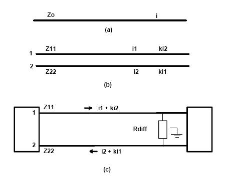
        图1(a)演示了一个典型的单根走线。其特征阻抗是Z0，其上流经的电流为i。沿线任意一点的电压为V=Z0*i（根据欧姆定律）。

        一般情况，线对：图1(b)演示了一对走线。线1具有特征阻抗Z11，与上文中Z0一致，电流i1。线2具有类似的定义。当我们将线2向线1靠近时，线2上的电流开始以比例常数k耦合到线1上。类似地，线1的电流i1开始以同样的比例常数耦合到线2上。每根走线上任意一点的电压，还是根据欧姆定律，为：

V1 = Z11*i1 + Z11*k*i2 （1）
V2 = Z22*i2 + Z22*k*i1

        现在我们定义Z12 = k*Z11以及Z21 = k*Z22。这样，式（1）就可以写成：

V1 = Z11*i1 + Z12*i2  （2）
V2 = Z21*i1 + Z22*i2

        这是一对熟悉的联立方程组，我们可以经常在教科书中看到。这个方程组可以推广到任意数量的走线，并且可以用你们中大部分人都熟悉的矩阵形式来表示。

        特殊情况，差分对：图1(c)演示了一对差分走线。重写式1：

V1 = Z11*i1 + Z11*k*i2 （1）
V2 = Z22*i2 + Z21*k*i1

        现在注意在仔细设计并且是对称的情况下，Z11 = Z22 = Z0，且i2 = -i1这将导致（经过一些变换）：

V1 = Z0*i1*(1-k)  （3）
V2 = -Z0*i1*(1-k)

        注意V1 = -V2，当然，这是我们已经知道的，因为这是一个差分对。

有效（差模）阻抗

        电压V1以地为参考。线1的有效阻抗（单独来看，在差分对中叫做“差模”阻抗，通常叫做“单线”阻抗）为电压除以电流，或：

Zodd = V1/i1 = Z0*(1-k)

        由上可知，因Z0 = Z11 且 k = Z12/Z11，上式可写成：Zodd = Z11 - Z12这也是一个在许多教科书中都可以看到的公式。

        为了防止反射，正确的端接方法是用一个值为Zodd的电阻。类似地，线2的差模阻抗与此相同（在对称差分对的特定情形下）。

差分阻抗

        假定在某一瞬间我们将两根走线用电阻端接到地。因为i1 = -i2，所以根本没有电流流经地。也就是说，没有真正的理由把电阻接地。事实上，有人认为，为了将差分信号和地噪声隔离，一定不能将它们接地。因此通常的连接形式如图1(c)中所示，用单个电阻连接线1与线2。电阻的值是线1和线2差模阻抗的和，或：

Zdiff  = 2*Z0*(1-k) 或
  2*(Z11 - Z12)

        这就是为什么你经常看到实际上一个差分对具有大约80Ω的差分阻抗，而每个单线阻抗是50Ω。

计算

        知道Zdiff是2*(Z11-Z12)不是很有用，因为Z12的值并不直观。但是，当我们看到Z12与耦合系数k有关，事情就变得清晰了。事实上，耦合系数与我在Brookspeak中关于串扰的专栏[1]中谈到的耦合系数是相同的。国家半导体发布的计算Zdiff的公式[2]已经被广泛接受：

Zdiff = 2*Z0(1-.48*e-.96*S/H)   微带线
Zdiff = 2*Z0(1-.347*e-2.9*S/H)  带状线

其中的术语在图2中定义。Z0为其传统定义[3] 。

 
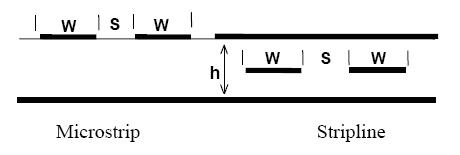
图 2 差分阻抗计算中的术语定义

共模阻抗

        为了讨论完整起见，共模阻抗与上面略有不同。第一个差别是i1 = i2（没有负号），这样式3就变成：

V1 = Z0*i1*(1+k) （4）
V2 = Z0*i1*(1+k)

        并且正如所期望的，V1 = V2。因此单线阻抗是Z0*(1+k)。在共模情况下，两根线的端接电阻均接地，所以流经地的电流为i1+i2且这两个电阻对器件表现为并联。也就是说，共模阻抗是这些电阻的并联组合，或：
Zcommon = (1/2)*Z0*(1+k)，或

Zcommon = (1/2)*(Z11 + Z12)

注意，这里差分对的共模阻抗大约为差模阻抗的1/4。