


- Python版本: Python3.x
- 运行平台: Windows
- IDE: jupyter / Colab
- 转载请标明出处:https://blog.csdn.net/tian121381/category_9748511.html
- 资料下载,提取码:rscg
前言
上一章,讲解了简单的神经网络和卷积,卷积中的过滤器究竟是什么样的呢?这章我们要来看一下,然后完成一下课后题,在细讲一个小程序就OK了
一、过滤器—补充
我们要通过在2D灰度图像上创建基本卷积来探索卷积如何工作。 首先,我们可以通过从scipy获取“ascent”图像来加载图像。 这是一张漂亮的内置图片,其中包含许多角度和线条。
导入相关包
import cv2
import tensorflow as tf
from scipy import misc
import numpy as np
import matplotlib.pyplot as plt
i = misc.ascent()  #misc模块自带一些灰度图像ascent和彩色的face图
设置图片格式,查看一下
plt.grid(False)   #网格线设置
plt.gray()
plt.axis("off") #不显示坐标尺寸
plt.imshow(i)
plt.show
结果:

该图像存储为一个numpy数组,因此我们只需复制该数组即可创建转换后的图像。 我们还要获取图像的尺寸,以便稍后进行循环。
i_transformed = np.copy(i)
size_x = i_transformed.shape[0]
size_y = i_transformed.shape[1]
#创建一个3*3的过滤器
#此滤镜可以很好地检测边缘
#它会产生仅通过尖锐边缘和笔直的卷积行

#不同的卷积行
#filter = [ [0, 1, 0], [1, -4, 1], [0, 1, 0]]
filter = [ [-1, -2, -1], [0, 0, 0], [1, 2, 1]]
#filter = [ [-1, 0, 1], [-2, 0, 2], [-1, 0, 1]]
#如果过滤器中的所有数字加起来都不为0或1,那么您可能应该进行权重操作,例如,如果您的权重为1,1,1 1,2,1 1,1,1。它们的总和为10,
#因此如果要对其进行归一化,则应将权重设置为.1。
weight  = 1
现在创建一个卷积。 我们将遍历图像,保留1个像素的空白,然后将当前像素的每个相邻像素乘以滤镜中定义的值。 也就是说,当前像素在其上方和左侧的邻居将与滤镜中的左上角项目等相乘。然后将结果乘以权重,然后确保结果在0-255范围内 最后,我们将新值加载到转换后的图像中。
for x in range(1,size_x-1):
  for y in range(1,size_y-1):
      convolution = 0.0
      convolution = convolution + (i[x - 1, y-1] * filter[0][0])
      convolution = convolution + (i[x, y-1] * filter[0][1])
      convolution = convolution + (i[x + 1, y-1] * filter[0][2])

      convolution = convolution + (i[x-1, y] * filter[1][0])
      convolution = convolution + (i[x, y] * filter[1][1])
      convolution = convolution + (i[x+1, y] * filter[1][2])
      convolution = convolution + (i[x-1, y+1] * filter[2][0])
      convolution = convolution + (i[x, y+1] * filter[2][1])
      convolution = convolution + (i[x+1, y+1] * filter[2][2])  #累加
      convolution = convolution * weight   #乘权重
      if(convolution<0):    #保证数据在0--255之间
        convolution=0
      if(convolution>255):
        convolution=255
      i_transformed[x, y] = convolution
查看运行后结果:
plt.gray()
plt.grid(False)
plt.imshow(i_transformed)
#plt.axis('off')
plt.show()
结果:

池化层大小是2x2。这里的理论是遍历图像,并查看上下左右,选取其中最大的一个并将其加载到新映像中。 因此,新图像的大小将是旧图像的1/4----通过此过程,X和Y的尺寸将减半。 会发现尽管进行了压缩,这些特征没有改变! 使图像的特征更加明显。
new_x = int(size_x/2)
new_y = int(size_y/2)
newImage = np.zeros((new_x, new_y))
for x in range(0, size_x, 2):
  for y in range(0, size_y, 2):
    pixels = []
    pixels.append(i_transformed[x, y])
    pixels.append(i_transformed[x+1, y])
    pixels.append(i_transformed[x, y+1])
    pixels.append(i_transformed[x+1, y+1])
    newImage[int(x/2),int(y/2)] = max(pixels)

# Plot the image. Note the size of the axes -- now 256 pixels instead of 512
plt.gray()
plt.grid(False)
plt.imshow(newImage)
#plt.axis('off')
plt.show()
结果:

可以看出,经过池化层处理后,特征更加明显了。
二、课后练习—CNN
通过上一章,我们了解了如何使用卷积来改进Fashion MNIST。
练习:请编写仅使用单个卷积层和单个MaxPooling 2D将MNIST的准确性提高到99.8%或更高。 一旦准确性超过此数量,您应该停止训练。 它应该在少于20个周期内发生,因此可以硬编码要训练的周期数是可以的,但是一旦达到上述指标,训练就结束。 如果不是,那么将需要重新设计图层。 达到99.8%时,您应该打印出字符串“达到99.8%的精度,因此取消训练!”
自写哈!!!
参考代码:
#导入相关包
import tensorflow as tf

#编写回调类
class MyCallbacks(tf.keras.callbacks.Callback):
    def on_epoch_end(self,epoch,logs={}):
        if(logs.get("accuracy") > 0.998):
            print("准确率大于99.8%,停止训练!")
            self.model.stop_training = True

#实例化
callbacks = MyCallbacks()
mnist = tf.keras.datasets.mnist

(training_images,training_labels),(test_images,test_labels) = mnist.load_data()
print(training_images.shape)   #60000 28 28
print(test_images.shape)       #10000,28,28

#数据处理
training_images = training_images.reshape(60000,28,28,1)
training_images = training_images/255
test_images = test_images.reshape(10000,28,28,1)
test_images = test_images/255

model = tf.keras.Sequential([
                            tf.keras.layers.Conv2D(16,(3,3),activation=tf.nn.relu,input_shape = (28,28,1)),
                            tf.keras.layers.MaxPool2D(2,2),
                            tf.keras.layers.Flatten(),
                            tf.keras.layers.Dense(128,activation='relu'),
                            tf.keras.layers.Dense(10,activation='softmax')
                            ])

model.compile(optimizer="adam",loss="sparse_categorical_crossentropy",metrics=["accuracy"])

model.fit(training_images,training_labels,epochs=20,callbacks=[callbacks])
结果:

#测试集测试
loss = model.evaluate(test_images,test_labels)
print("损失值:",loss[0],"\n精度:",loss[1
结果:
10000/10000 [==============================] - 1s 62us/sample - loss: 0.0796 - accuracy: 0.9800
损失值: 0.07962530491302118
精度: 0.98
三、实例细讲CNN
这里的内容,我使用的IDE是Colab,如下图,有FanQ上网条件的同学可以试一下,很好用的,是谷歌的一个网页版编译器,可以免费使用谷歌的GUP。没有的同学用jupyter和pycharm都可以。

小废话
如果使用的是colab,需要先运行以下代码
from google.colab import drive
drive.mount('/content/drive')
会给你一个链接

点进链接,登录谷歌账号,会给一个授权码code,将它放入运行框中,回车即可链接谷歌云盘成功,数据都在谷歌云盘保存。
导入数据
我有一组人和马的数据集,想要通过卷积模型,来判断我再次输入的图片是人还是马。开始吧
以下python代码将使用OS库来使用操作系统库,从而使您可以访问文件系统,并使用zipfile库来解压缩数据。(数据放在置顶资料下载处)
import os
import zipfile
import matplotlib.pyplot as plt
import matplotlib.image as mpimg
local_zip = 'Dataset/horse-or-human.zip'
#读文件
zip_ref = zipfile.ZipFile(local_zip, 'r')
 #解压到
zip_ref.extractall('tmp/horse-or-human')
local_zip = 'Dataset/validation-horse-or-human.zip'
zip_ref =zipfile.ZipFile(local_zip,'r')
zip_ref.extractall('tmp/validation-horse-or-human')
zip_ref.close()
zip的内容被提取到基本目录/ tmp / horse-or-human,而每个目录又包含马和人的子目录。 简而言之:训练集是用于告诉神经网络模型“这就是马的样子”,“这就是人的样子”的数据。
此示例中要注意的一件事:我们没有将图像明确标记为马或人。 如果您还记得上面的手写示例,我们将其标记为“这是1”,“这是7”等。稍后,您将看到正在使用的称为ImageGenerator的东西—编码为从子目录读取图像, 并从该子目录的名称中自动标记它们。 因此,例如,您将拥有一个“培训”目录,其中包含一个“马”目录和一个“人”目录。 ImageGenerator将为您适当地标记图像,从而减少了编码步骤。 让我们定义以下每个目录:
#马的训练集文件夹
train_horse_dir = os.path.join('tmp/horse-or-human/horses')
#人的训练集文件夹
train_human_dir = os.path.join('tmp/horse-or-human/humans')

#验证集
validation_horse_dir = os.path.join('tmp/validation-horse-or-human/horses')
validation_human_dir = os.path.join('tmp/validation-horse-or-human/humans')
现在,看看马匹和人类训练目录中的文件名是什么样的:
#输出前10个文件名
train_horse_names = os.listdir(train_horse_dir)   #文件名列表
print(train_horse_names[:10])

train_human_names = os.listdir(train_human_dir)
print(train_human_names[:10])
结果:
['horse41-2.png', 'horse05-6.png', 'horse31-9.png', 'horse42-9.png', 'horse28-8.png', 'horse45-7.png', 'horse21-8.png', 'horse46-0.png', 'horse31-4.png', 'horse25-1.png']
['human04-27.png', 'human13-23.png', 'human17-18.png', 'human17-09.png', 'human03-20.png', 'human16-15.png', 'human14-09.png', 'human02-14.png', 'human05-15.png', 'human07-15.png']
目录中的马和人像总数(训练集和验证集):
print('total training horse images:', len(os.listdir(train_horse_dir)))
print('total training human images:', len(os.listdir(train_human_dir)))
print('total validation_horse images:', len(os.listdir(validation_horse_dir)))
print('total validation_human images:', len(os.listdir(validation_human_dir)))在这里插入代码片
结果:
total training horse images: 500
total training human images: 527
total validation_horse images: 500
total validation_human images: 527
现在,看一些图片,以更好地了解它们。 首先,配置matplot参数:
#以4x4输出图像
nrows = 4
ncols = 4
# 遍历图像的索引
pic_index = 0
#设置matplotlib,并调整其大小以适合4x4图片
fig = plt.gcf()   #获取当前图的参考。
# 显示出8个马,8个人
fig.set_size_inches(nrows*4,ncols*4)
pic_index += 8
next_horse_pix = [os.path.join(train_horse_dir, fname)
                for fname in train_horse_names[pic_index-8:pic_index]]
next_human_pix = [os.path.join(train_human_dir, fname)
                for fname in train_human_names[pic_index-8:pic_index]]

for i, img_path in enumerate(next_horse_pix+next_human_pix):   #总个数
  # Set up subplot; subplot indices start at 1
  sp = plt.subplot(nrows, ncols, i + 1)
  sp.axis('Off') # Don't show axes (or gridlines)

  img = mpimg.imread(img_path)
  plt.imshow(img)
plt.show()
结果:

模型的构建
数据我们都处理好了,那么就到了模型这一步了。
#导入相关包
import tensorflow as tf
然后,像前面的示例一样,添加卷积层,并将最终结果展平以输入连接的层。 最后,我们添加全连接层。 请注意,由于我们面临两类分类问题,即二进制分类问题,因此我们将以sigmoid activation型激活来结束网络,以便网络的输出将是介于0和1之间的单个标量,从而编码 当前图像是1类(而不是0类)。
#模型
model = tf.keras.Sequential([tf.keras.layers.Conv2D(16,(3,3),activation="relu",input_shape = (300,300,3)),
                             tf.keras.layers.MaxPool2D(2,2),

                             tf.keras.layers.Conv2D(32,(3,3),activation="relu"),
                             tf.keras.layers.MaxPool2D(2,2),

                             tf.keras.layers.Conv2D(64,(3,3),activation="relu"),
                             tf.keras.layers.MaxPool2D(2,2),
                             tf.keras.layers.Conv2D(64,(3,3),activation="relu"),
                             tf.keras.layers.MaxPool2D(2,2),
                             tf.keras.layers.Conv2D(64,(3,3),activation="relu"),
                             tf.keras.layers.MaxPool2D(2,2),

                             tf.keras.layers.Flatten(),
                             tf.keras.layers.Dense(512,activation="relu"),
                             tf.keras.layers.Dense(1,activation="sigmoid")
                            ])
调用model.summary()来看一下网络的具体结构。

“Output_Shape”列显示了图像的大小在每个连续的图层中如何演变。 卷积层由于填充而使特征图的大小略微减少,每个池化层将尺寸减半。
接下来,我们将配置模型训练的规范。 使用binary_crossentropy损失训练模型,因为这是一个二进制分类问题,而我们的最终激活是sigmoid。 使用rmsprop优化器,其学习率为0.001。 在训练期间,我们将要监控分类的准确性。
注意:在这种情况下,使用RMSprop优化算法要优于随机梯度下降(SGD),因为RMSprop可以自动为我们调整学习速率。(其他优化器,例如Adam和Adagrad,也可以在训练过程中自动调整学习率,并且在此处同样适用。)
from tensorflow.keras.optimizers import RMSprop
model.compile(optimizer=RMSprop(lr = 0.001),loss="binary_crossentropy",metrics=["accuracy"])
数据预处理
设置数据生成器,该数据生成器将读取源文件夹中的图片,将其转换为float32张量,并将它们(带有标签)送到我们的网络中。我们将为训练图像提供一个生成器,为验证图像提供一个生成器。生成器将生成一批尺寸为300x300的图像及其标签(二进制)。
进入神经网络的数据通常应该以某种方式进行规范化,以使其更适合网络处理。 (将原始像素输入到卷积图中是很罕见的。)在本例中,我们将通过将像素值标准化为[0,1]范围(最初所有值都在[0,255]范围内)来预处理图像)。
在Keras中,这可以通过keras.preprocessing.image.ImageDataGenerator类使用rescale参数来完成。使用此ImageDataGenerator类,可以通过 .flow(data, labels)或 .flow_from_directory(directory) 实例化增强图像批处理(及其标签)的生成器。然后,这些生成器可以与Keras模型方法一起使用,这些方法将数据生成器作为输入:fit_generator,evaluate_generator和predict_generator。
from tensorflow.keras.preprocessing.image import ImageDataGenerator   #导入图片生成器
#归一化
train_datagen = ImageDataGenerator(rescale=1/255)
validation_datagen = ImageDataGenerator(rescale=1/255)
#使用train_datagen生成器分批流训练图像128
train_generator = train_datagen.flow_from_directory(
    'tmp/horse-or-human/',
    target_size = (300,300),   #重置图片大小
    batch_size = 128,
    class_mode = 'binary'   #二进制,模型选择binary
)
#使用train_datagen生成器分批流验证图像128
validation_generator = validation_datagen.flow_from_directory(
        'tmp/validation-horse-or-human/',  # This is the source directory for training images
        target_size=(300, 300),  # All images will be resized to 150x150
        batch_size=32,
        # Since we use binary_crossentropy loss, we need binary labels
        class_mode='binary')
结果:
Found 1027 images belonging to 2 classes.
Found 1027 images belonging to 2 classes.
可以看出训练集和测试集都是1027个图片,共两类。
开始训练
- 训练15个周期
- 注意每个时期的值。
- 损失和准确性是训练进度的重要标志。它正在猜测训练数据的分类,然后根据已知标签对其进行测量,然后计算结果。准确性是正确猜测的一部分。
model.fit_generator(
    train_generator,    #训练集,使用训练集的图像生成器
    steps_per_epoch = 8,#训练集共1024个图象,每次载入128,共8批
    epochs = 15,
    verbose = 1,
    validation_data = validation_generator,  #共256
    validation_steps = 8   #每次32,共8批
    )

注:我这里是GPU跑的,速度会较快,和我运行时间相差太多,不要怀疑数据或模型错误。
模型训练好后,我们就再网上下载几个马,人的图片,放入模型,看看结果。
运行模型
(这里用不了colab的可以跳过,看我的结果,也可以自己处理图片放入模型)
现在让我们看一下使用模型实际运行预测。 此代码将允许您从文件系统中选择1个或多个文件,然后将其上传并在模型中运行它们,从而指示对象是马还是人。
我在网上下载图片如下:

import numpy as np
from google.colab import file
from keras_preprocessing import image

uploaded = files.upload()
for fn in uploaded.keys():
  # 预测图片
  path = '/content/' + fn    #预测图片的位置
  img = image.load_img(path,target_size=(300,300))
  x = image.img_to_array(img)
  x = np.expand_dims(x,axis=0)

  images = np.vstack([x])
  classes = model.predict(images, batch_size=10)
  print(classes[0])
  if classes[0]>0.5:
    print(fn + " is a human")
  else:
    print(fn + " is a horse")

我们上传成功,也可以看到预测结果人。
第二个图呢?

可以看到也是成功的预测出bbb.jpg是马。
中间各层的可视化
为了感觉一下我们的卷积网络学习了哪些功能,要做的一件有趣的事情是可视化输入在卷积网络中的转换方式。 让我们从训练集中选择一个随机图像,然后生成一个图形,其中每一行都是图层的输出,而行中的每一幅图像都是该输出要素图中的特定过滤器。 重新运行此单元格以生成各种训练图像的中间表示。
import numpy as np
import random
from tensorflow.keras.preprocessing.image import img_to_array, load_img

#定义一个新模型,该模型将图像作为输入,并在第一个模型之后输出先前模型中所有层的中间表示。
successive_outputs = [layer.output for layer in model.layers[1:]]

#visualization_model = Model(img_input, successive_outputs)
visualization_model = tf.keras.models.Model(inputs = model.input, outputs = successive_outputs)

#从训练集中准备一个随机的输入图像。
horse_img_files = [os.path.join(train_horse_dir, f) for f in train_horse_names]
human_img_files = [os.path.join(train_human_dir, f) for f in train_human_names]
img_path = random.choice(horse_img_files + human_img_files)

img = load_img(img_path, target_size=(300, 300))
x = img_to_array(img)  # Numpy array with shape (300, 300, 3)
x = x.reshape((1,) + x.shape)  # Numpy array with shape (1, 300, 300, 3)

# 归一化
x /= 255

#通过网络运行图像,从而获得该图像的所有中间表示。
successive_feature_maps = visualization_model.predict(x)

# 这些是图层的名称,因此可以将其作为绘图的一部分
layer_names = [layer.name for layer in model.layers]

for layer_name, feature_map in zip(layer_names, successive_feature_maps):
  if len(feature_map.shape) == 4:
    # 仅对conv / maxpool层执行此操作,而不对完全连接的层执行此操作
    n_features = feature_map.shape[-1]  # 图中的特征数量
    # 图像的形状 (1, size, size, n_features)
    size = feature_map.shape[1]
    # 在此矩阵中平铺图像
    display_grid = np.zeros((size, size * n_features))
    for i in range(n_features):
      # 处理特征使其可视化
      x = feature_map[0, :, :, i]
      x -= x.mean()
      x /= x.std()
      x *= 64
      x += 128
      x = np.clip(x, 0, 255).astype('uint8')
      # 将每个滤镜平铺到这个大的水平网格中
      display_grid[:, i * size : (i + 1) * size] = x
    # 显示网格
    scale = 20. / n_features
    plt.figure(figsize=(scale * n_features, scale))
    plt.title(layer_name)
    plt.grid(False)
    plt.imshow(display_grid, aspect='auto', cmap='viridis')

正如所见,我们从图像的原始像素过渡到越来越抽象和紧凑的表示形式。 下面的表示开始突出显示网络要注意的内容,并且显示“激活”的功能越来越少。 大多数设置为零。 这称为“稀疏”。 表示稀疏性是深度学习的关键特征。 这些表示所携带的关于图像原始像素的信息越来越少,但是携带的有关图像类别的信息却越来越精细。 可以将卷积网络(或通常称为深层网络)视为信息蒸馏管道。
清理内存
在运行下一个程序之前,运行以下单元格以终止内核并释放内存资源。(colab)
import os, signal
os.kill(os.getpid(), signal.SIGKILL)
四、课后练习
该数据集包含80张图像,40张快乐的和40张悲伤的图像。 创建一个在这些图像上训练达到100%准确度的卷积神经网络,当达到>0 .999的训练准确度时将取消训练。
提示—最好在3个卷积层上使用。
参考代码:
#使用Colab的,先运行这段代码---获取授权码--加载云盘-----------------
from google.colab import drive
drive.mount('/content/drive')
#-----------------------------------
#导入相关包
import tensorflow as tf
import zipfile
import matplotlib.pyplot as plt
import matplotlib.image as mpimg
from tensorflow.keras.optimizers import RMSprop
#导入图片生成器,处理图片数据
from tensorflow.keras.preprocessing.image import ImageDataGenerator
import os

#数据集位置
local_zip = '/content/drive/My Drive/Colab Notebooks/DateSet/happy-or-sad.zip'
#读取文件
zip_ref = zipfile.ZipFile(local_zip,'r')
#解压到指定文件夹
zip_ref.extractall("tmp/happy-or-sad")
zip_ref.close()
#数据处理完成,后面创建回溯函数,按要求停止。
class myCallback(tf.keras.callbacks.Callback):
  def on_epoch_end(self,epoch,logs={}):
    if(logs.get("acc") > 0.999):
      print("准确率到达99。9%,停止训练!")
      self.model.stop_training = True
#实例化
callbacks = myCallback()
#编写网络模型、
model = tf.keras.Sequential([
                tf.keras.layers.Conv2D(32,(3,3,),activation="relu",input_shape = (300,300,3)),
                tf.keras.layers.MaxPool2D(2,2),


                tf.keras.layers.Conv2D(64,(3,3,),activation="relu"),
                tf.keras.layers.MaxPool2D(2,2),

                tf.keras.layers.Conv2D(64,(3,3,),activation="relu"),
                tf.keras.layers.MaxPool2D(2,2),

                tf.keras.layers.Flatten(),
                tf.keras.layers.Dense(512,activation="relu"),
                #二分类,输出一类结果
                tf.keras.layers.Dense(1,activation="sigmoid")  ])
#查看一下模型结构
#model.summary()
#设置优化,和损失计算方法
model.compile(optimizer=RMSprop(lr=0.001),loss="binary_crossentropy",metrics=["accuracy"])
#图片像素0--255,使用ImageDataGenerator对图片数据规范化
train_datagen = ImageDataGenerator(rescale = 1/255)
#使用train_datagen生成器分批处理训练图片
train_generate = train_datagen.flow_from_directory(
    "/content/tmp/happy-or-sad/",
    target_size = (300,300),
    batch_size = 16,
    class_mode = "binary" )

"""
Found 80 images belonging to 2 classes.
"""
#开始训练
model.fit_generator(train_generate,
          steps_per_epoch = 5,#训练集共80个图象,每次载入16,共5批
          epochs = 15, #迭代15次
          verbose = 1,
          callbacks = [callbacks]
          )
结果:

训练完成
看一下实际的分类怎么样?(选作)
我这用的Colab,没有的同学们也可以自己写图片处理的代码,验证一下。
import numpy as np
from google.colab import files
from keras_preprocessing import image
uploaded = files.upload()
for fn in uploaded.keys():
  # 预测图片
  path = '/content/' + fn    #预测图片的位置
  img = image.load_img(path,target_size=(300,300))
  x = image.img_to_array(img)
  x = np.expand_dims(x,axis=0)

  images = np.vstack([x])
  classes = model.predict(images, batch_size=10)
  print(classes[0])

  if classes[0]>0.5:
    print(fn + " is happy")
  else:
    print(fn + " is sad")
我给的图片是

结果:
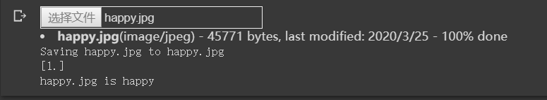
可以看到结果正确。
五、结语
这章,我们通过了一个实例讲解了CNN。然后留了一个课后练习,自己完成后,再看我的哈!
- 如有错误,请不吝指教,谢谢!(❤ ω ❤)
- 这章就先到这里吧,下节见!(ง •_•)ง


 被折叠的 条评论
为什么被折叠?
被折叠的 条评论
为什么被折叠?
 到【灌水乐园】发言


