tensorflow2_tf.keras实现softmax多分类以及网络优化与超参数选择

自动下载训练图像，我这里print输出了大小

import tensorflow as tf
import pandas as pd
import numpy as np
import matplotlib.pyplot as plt
#加载数据集
(train_image, train_lable), (test_image, test_label) = tf.keras.datasets.fashion_mnist.load_data()
print('train_image.shape', train_image.shape)
print('test_image.shape', test_image.shape)
print('train_lable', train_lable)

运行结果：

Downloading data from https://storage.googleapis.com/tensorflow/tf-keras-datasets/train-labels-idx1-ubyte.gz
32768/29515 [=================================] - 0s 2us/step
40960/29515 [=========================================] - 0s 2us/step
Downloading data from https://storage.googleapis.com/tensorflow/tf-keras-datasets/train-images-idx3-ubyte.gz
26427392/26421880 [==============================] - 4s 0us/step
26435584/26421880 [==============================] - 4s 0us/step
Downloading data from https://storage.googleapis.com/tensorflow/tf-keras-datasets/t10k-labels-idx1-ubyte.gz
16384/5148 [===============================================================================================] - 0s 0s/step
Downloading data from https://storage.googleapis.com/tensorflow/tf-keras-datasets/t10k-images-idx3-ubyte.gz
4423680/4422102 [==============================] - 1s 0us/step
4431872/4422102 [==============================] - 1s 0us/step
train_image.shape (60000, 28, 28)
test_image.shape (10000, 28, 28)
train_lable [9 0 0 ... 3 0 5]

Process finished with exit code 0

自动下载的数据集，速度还是可以的。

对数据进行归一化处理，像素范围是0到255，所以都除以255，归一化到（0，1）之间

train_image = train_image/255
test_image = test_image/255

然后：

构建网络，构建个什么样的网络呢？

先从含有一个隐藏层的简单网络开始吧，隐藏层神经元为多少合适呢？

由于输入数据包含很多信息所以神经元个数不能太少，太少的化会丢弃很多有用的信息，暂定为64。

model = tf.keras.Sequential()
#添加Flatten层将（28，28）的数据变成[28*28]
model.add(tf.keras.layers.Flatten(input_shape=(28, 28)))
model.add(tf.keras.layers.Dense(64, activation='relu'))
model.add(tf.keras.layers.Dense(10, activation='softmax'))
model.summary()

下一步，设置优化器和损失函数，用常用的adam优化器， Adam算法通常被认为对超参数的选择相当鲁棒 ，可以看做是修正后的Momentum+RMSProp算法，学习率建议为0.001。

softmax的损失函数有两种：

categorical_crossentropy  label为one hot 编码时使用

sparse_categorical_crossentropy 我们数据集的label是0到9的数字，不是one hot 编码，所以我们此处选它。

model.compile(optimizer = 'adam',
              loss = 'sparse_categorical_crossentropy',
              metrics=['acc']
)

现在终于可以训练了

history = model.fit(train_image,train_lable,epochs=20)

 训练结果

Epoch 1/20
1875/1875 [==============================] - 1s 583us/step - loss: 2.2495 - acc: 0.6383
Epoch 2/20
1875/1875 [==============================] - 1s 569us/step - loss: 0.7981 - acc: 0.6904
Epoch 3/20
1875/1875 [==============================] - 1s 566us/step - loss: 0.7040 - acc: 0.7149
Epoch 4/20
1875/1875 [==============================] - 1s 569us/step - loss: 0.6420 - acc: 0.7429
Epoch 5/20
1875/1875 [==============================] - 1s 564us/step - loss: 0.5893 - acc: 0.7785
Epoch 6/20
1875/1875 [==============================] - 1s 571us/step - loss: 0.5584 - acc: 0.8034
Epoch 7/20
1875/1875 [==============================] - 1s 569us/step - loss: 0.5341 - acc: 0.8141
Epoch 8/20
1875/1875 [==============================] - 1s 573us/step - loss: 0.5255 - acc: 0.8189
Epoch 9/20
1875/1875 [==============================] - 1s 582us/step - loss: 0.5156 - acc: 0.8205
Epoch 10/20
1875/1875 [==============================] - 1s 579us/step - loss: 0.5116 - acc: 0.8242
Epoch 11/20
1875/1875 [==============================] - 1s 574us/step - loss: 0.5148 - acc: 0.8244
Epoch 12/20
1875/1875 [==============================] - 1s 580us/step - loss: 0.5036 - acc: 0.8281
Epoch 13/20
1875/1875 [==============================] - 1s 582us/step - loss: 0.4950 - acc: 0.8306
Epoch 14/20
1875/1875 [==============================] - 1s 579us/step - loss: 0.4987 - acc: 0.8308
Epoch 15/20
1875/1875 [==============================] - 1s 576us/step - loss: 0.4899 - acc: 0.8332
Epoch 16/20
1875/1875 [==============================] - 1s 578us/step - loss: 0.4907 - acc: 0.8322
Epoch 17/20
1875/1875 [==============================] - 1s 579us/step - loss: 0.4854 - acc: 0.8343
Epoch 18/20
1875/1875 [==============================] - 1s 575us/step - loss: 0.4829 - acc: 0.8355
Epoch 19/20
1875/1875 [==============================] - 1s 571us/step - loss: 0.4952 - acc: 0.8342
Epoch 20/20
1875/1875 [==============================] - 1s 570us/step - loss: 0.4769 - acc: 0.8369

Process finished with exit code 0

打印训练过程

plt.plot(history.epoch, history.history.get('acc'))
plt.xlabel('epochs')
plt.ylabel('acc')

显示

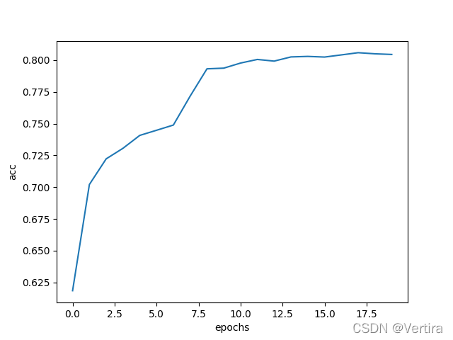
 图1

下面在第一个model的基础上增加隐藏层，增加1个吧，epoch还是20

这次是完整的代码2，与上面的代码1有些不同：（上面的代码合起来也是完整的代码1,）

import tensorflow as tf
import pandas as pd
import numpy as np
import matplotlib.pyplot as plt
#加载数据集
(train_image, train_lable), (test_image, test_label) = tf.keras.datasets.fashion_mnist.load_data()
# print('train_image.shape', train_image.shape)
# print('test_image.shape', test_image.shape)
# print('train_lable', train_lable)
# plt.imshow(train_image[1])

model = tf.keras.Sequential()
#添加Flatten层将（28，28）的数据变成[28*28]
model.add(tf.keras.layers.Flatten(input_shape=(28, 28)))
model.add(tf.keras.layers.Dense(64, activation='relu'))
model.add(tf.keras.layers.Dense(64, activation='relu'))
model.add(tf.keras.layers.Dense(10, activation='softmax'))
model.summary()

model.compile(optimizer='adam',
              loss='sparse_categorical_crossentropy',
              metrics=['acc']
)
history = model.fit(train_image, train_lable, epochs=20)

# print('history.history.get()', history.history.get('acc'))
# print('history.epoch', history.epoch)

plt.plot(history.epoch, history.history.get('acc'))
plt.xlabel('epochs')
plt.ylabel('acc')
plt.show()

训练结果：

Epoch 1/20
1875/1875 [==============================] - 1s 618us/step - loss: 1.8487 - acc: 0.7279
Epoch 2/20
1875/1875 [==============================] - 1s 622us/step - loss: 0.6725 - acc: 0.7880
Epoch 3/20
1875/1875 [==============================] - 1s 622us/step - loss: 0.5984 - acc: 0.8011
Epoch 4/20
1875/1875 [==============================] - 1s 618us/step - loss: 0.5592 - acc: 0.8081
Epoch 5/20
1875/1875 [==============================] - 1s 613us/step - loss: 0.5271 - acc: 0.8198
Epoch 6/20
1875/1875 [==============================] - 1s 621us/step - loss: 0.4961 - acc: 0.8294
Epoch 7/20
1875/1875 [==============================] - 1s 621us/step - loss: 0.4764 - acc: 0.8351
Epoch 8/20
1875/1875 [==============================] - 1s 626us/step - loss: 0.4458 - acc: 0.8430
Epoch 9/20
1875/1875 [==============================] - 1s 621us/step - loss: 0.4292 - acc: 0.8457
Epoch 10/20
1875/1875 [==============================] - 1s 626us/step - loss: 0.4058 - acc: 0.8536
Epoch 11/20
1875/1875 [==============================] - 1s 612us/step - loss: 0.3965 - acc: 0.8563
Epoch 12/20
1875/1875 [==============================] - 1s 621us/step - loss: 0.3873 - acc: 0.8587
Epoch 13/20
1875/1875 [==============================] - 1s 626us/step - loss: 0.3777 - acc: 0.8619
Epoch 14/20
1875/1875 [==============================] - 1s 620us/step - loss: 0.3831 - acc: 0.8611
Epoch 15/20
1875/1875 [==============================] - 1s 628us/step - loss: 0.3717 - acc: 0.8652
Epoch 16/20
1875/1875 [==============================] - 1s 685us/step - loss: 0.3669 - acc: 0.8656
Epoch 17/20
1875/1875 [==============================] - 1s 704us/step - loss: 0.3666 - acc: 0.8676
Epoch 18/20
1875/1875 [==============================] - 1s 714us/step - loss: 0.3608 - acc: 0.8693
Epoch 19/20
1875/1875 [==============================] - 1s 666us/step - loss: 0.3582 - acc: 0.8682
Epoch 20/20
1875/1875 [==============================] - 1s 645us/step - loss: 0.3581 - acc: 0.8690

图像显示：

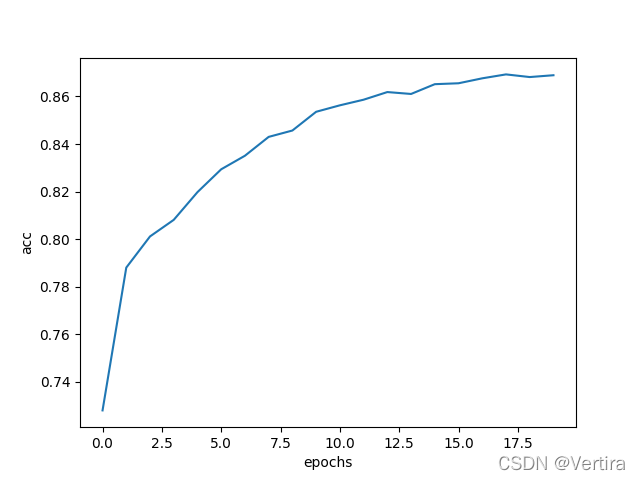
 图2

acc与图1有所提高。

下面看看测试集上的表现

model.evaluate(test_image,test_label)

 [0.4646746516227722, 0.8414000272750854]

acc 只有0.8414