CS224N assignment 1

来学NLP, 课程是斯坦福CS224N, 我用的2021版, b站搜出来的第一个就是了

• 课程网站：Stanford CS 224N | Natural Language Processing with Deep Learning

• 课程视频：【斯坦福CS224N】(2021|中英) 深度自然语言处理Natural Language Processing with Deep Learning_哔哩哔哩_bilibili

• 课程教材：无

• 课程作业：Stanford CS 224N | Natural Language Processing with Deep Learning，5 个编程作业 + 1 个 Final Project

• assignment 1 文件下载链接:http://web.stanford.edu/class/cs224n/assignments/a1.zip

• assignment 1 说明网址: exploring_word_vectors_22_23 (stanford.edu)

• Anaconda 网站链接: Free Download | Anaconda

观前提醒

1. 机翻存在

2. 本人菜逼

准备工作

• 确认python版本

  • win + r, 输入cmd打开终端, 输入python查看python版本, 需要确保版本在3.5以上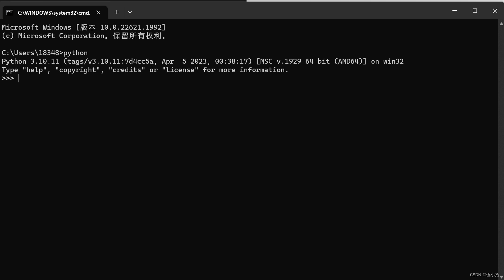

    

• 安装Anaconda

  • 网站链接: Free Download | Anaconda

  • 直接官网下载一路向下就好了

    

• 配置运行环境

  • 安装conda之后，关闭所有可能打开的终端。然后打开一个新的终端，运行以下命令:

  • 创建一个环境，并在env.yml中指定依赖项(记得把a1文件夹里的env.yml拖进去):

     conda env create -f env.yml

  • 激活新环境:

     conda activate cs224n

  • 在新的环境中，安装IPython内核，这样我们就可以在jupyter中使用这个环境:

     python -m ipykernel install --user --name cs224n

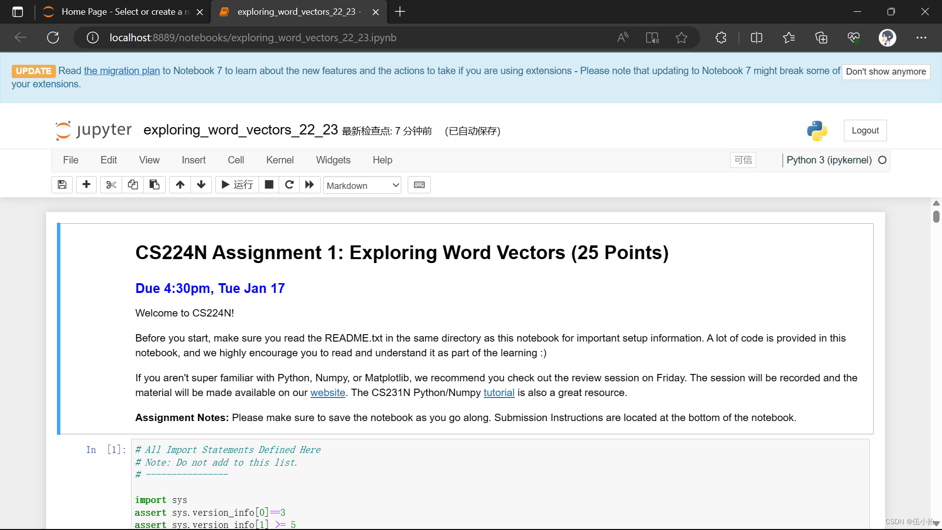
  • 作业1(仅限)是一本Jupyter Notebook。完成上述操作后，您应该可以通过输入下面的代码来获取underway(记得把a1文件夹里的exploring_word_vectors.ipynb拖进去):

     jupyter notebook exploring_word_vectors.ipynb

    现在应该打开的是一个网页, 里面是本次作业的要求

    

  • 为了确保我们使用了正确的环境，转到exploring_word_vectors.ipynb的工具栏，点击Kernel ->Change kernel，您应该能在下拉菜单中看到并选择cs224n。

  • 备注1:要停用一个正在运行的环境，使用

     conda deactivate

  • 备注2: 终端输入conda指令报错'conda' 不是内部或外部命令，也不是可运行的程序或批处理文件。

    终端输入path可以看到电脑配置的环境变量, 有可能会发现anaconda和scripts没有加进去

    我的电脑---右键属性---高级系统设置---环境变量---系统变量---Path---双击进入---新建---浏览---找到Anaconda和Scripts的路径添加，然后点击确定就好了。

    现在在命令行输入以下代码就可以看见conda版本了

     conda --version

作业

词向量

词向量通常被用作下游NLP任务的基本组件，例如问答，文本生成，翻译等，因此建立一些关于其优缺点的感知是很重要的。在这里，你将探索两种类型的词向量:来自共现矩阵(cooccurrence matrices)的词向量和来自GloVe的词向量。

术语说明:术语“词向量(word vectors)”和“词嵌入(word embeddings)”通常可以互换使用。术语“嵌入”指的是我们在较低维度空间中编码单词含义的各个方面。正如维基百科所述，“从概念上讲，它涉及到从一个一维的空间到一个低维的连续向量空间的数学嵌入(conceptually it involves a mathematical embedding from a space with one dimension per word to a continuous vector space with a much lower dimension)”。

Part 1: Count-Based Word Vectors (10 points)

大多数词向量模型都是从以下想法开始的:

You shall know a word by the company it keeps (Firth, J. R. 1957:11)

许多词向量实现都是由类似的词(即(近似)同义词)将在类似的上下文中使用的想法驱动的。因此，相似的单词通常在被说或写的时候会伴随着一个共同的单词子集，即上下文。通过检查这些上下文，我们可以尝试为我们的单词开发嵌入。有了这种直觉，许多构建词向量的“老派”方法依赖于词计数。在这里，我们详细介绍其中一种策略，即共现矩阵(co-occurrence matrices)(有关更多信息，请参阅此处或此处)。

Co-Occurrence

共现矩阵计算事物在某些环境中共现的频率。给定文档中出现的某个单词w_i，我们考虑围绕w_i的上下文窗口。假设我们的固定窗口大小为n，那么这就是该文档中n前面和n后面的单词，即单词w_{i-n} \dots w_{i-1}和w_{i+1} \dots w_{i+n}。我们构建一个共现矩阵 M，它是一个对称的逐字矩阵，其中M_{ij}是在所有文档中w_j出现在w_i的窗口内的次数。

Example: 固定窗口大小n=1的共现矩阵:

Document 1: "all that glitters is not gold"

Document 2: "all is well that ends well"

*	<START>	all	that	glitters	is	not	gold	well	ends	<END>
<START>	0	2	0	0	0	0	0	0	0	0
all	2	0	1	0	1	0	0	0	0	0
that	0	1	0	1	0	0	0	1	1	0
glitters	0	0	1	0	1	0	0	0	0	0
is	0	1	0	1	0	1	0	1	0	0
not	0	0	0	0	1	0	1	0	0	0
gold	0	0	0	0	0	1	0	0	0	1
well	0	0	1	0	1	0	0	0	1	1
ends	0	0	1	0	0	0	0	1	0	0
<END>	0	0	0	0	0	0	1	1	0	0

注:在NLP中，我们经常添加<START>和 <END> 标记来表示句子、段落或文档的开始和结束。在这种情况下，我们用<START>和<END> 标记封装每个文档，例如，<START>all that glitters is not gold<END> ，并将这些标记包含在我们的共现计数中。

这个矩阵的行(或列)提供了一种类型的词向量(基于词-词共出现的向量)，但是这些向量通常很大(语料库中不同词的数量呈线性)。因此，我们的下一步是进行降维(dimensionality reduction)。特别地，我们将运行SVD(Singular Value Decomposition)，这是一种广义的PCA (Principal Components Analysis)来选择最上面的k主成分。这是SVD的降维可视化。在这张图中，我们的共现矩阵是A，其中n行对应n个单词。我们得到了一个完整的矩阵分解，其中奇异值在对角线S矩阵中排序，以及我们新的，更短的长度为k的词向量在U_k中。

笔者注: 这个可能有点看不明白, 需要线性代数的一些知识(好吧我线性代数的知识都还给老师了), 所以贴一个链接

奇异值分解（SVD） - 知乎 (zhihu.com)

【学长小课堂】什么是奇异值分解SVD--SVD如何分解时空矩阵哔哩哔哩bilibili

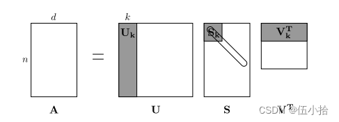
这种降维共现表示保留了单词之间的语义关系，例如，医生和医院将比医生和狗更接近。

注:如果你几乎不记得特征值是什么，这里有一个SVD介绍。如果您想更深入地了解PCA或SVD，请随时查看CS168的讲座7、8和9。这些课程笔记提供了对这些通用算法的高级处理。不过，就本课程而言，您只需要知道如何通过从numpy、scipy或sklearn python包中利用这些算法的预编程实现来提取k维嵌入。在实践中，由于执行PCA或SVD需要内存，因此将完整的SVD应用于大型语料库是具有挑战性的。但是，如果您只想要相对较小的k的前k向量组件-称为Truncated SVD -那么有合理的可扩展技术来迭代地计算这些组件。

Plotting Co-Occurrence Word Embeddings

在这里，我们将使用路透社(商业和金融新闻)语料库。如果您还没有运行本页顶部的导入单元格，请现在运行它(单击它并按SHIFT-RETURN键)。该语料库包含10788个新闻文档，共计130万字。这些文档跨越90个类别，分为训练和测试。欲了解更多详情，请访问https://www.nltk.org/book/ch02.html。我们在下面提供了一个“read_corpus”函数，它只从“黄金”类别中提取文章(即关于黄金，采矿等的新闻文章)。该函数还向每个文档添加<START>和 <END> 标记，以及小写单词。您不需要执行任何其他类型的预处理。

 def read_corpus(category="gold"):
     """ Read files from the specified Reuter's category.
         Params:
             category (string): category name
         Return:
             list of lists, with words from each of the processed files
     """
     files = reuters.fileids(category)
     return [[START_TOKEN] + [w.lower() for w in list(reuters.words(f))] + [END_TOKEN] for f in files]
 ​

解释以下上面的代码(好吧其实就是翻译以下注释)

• 从指定的reuters分类中读取文件

• 参数

  • category(字符串): 目录名称

• 返回

  • 二位数组，包含每个已处理文件中的单词

    • START_TOKEN/ [END_TOKEN]: 之前的<start>和<end>标志

    • 二维数组里的每一个单独的数组都是这样的一个结构[START_TOKEN] + [w.lower() for w in list(reuters.words(f))] + [END_TOKEN]

    • 也就是reuters.words(f)里所有单词的小写(lower函数返回字符串小写)

    • f是文件列表, 所以是for f in files

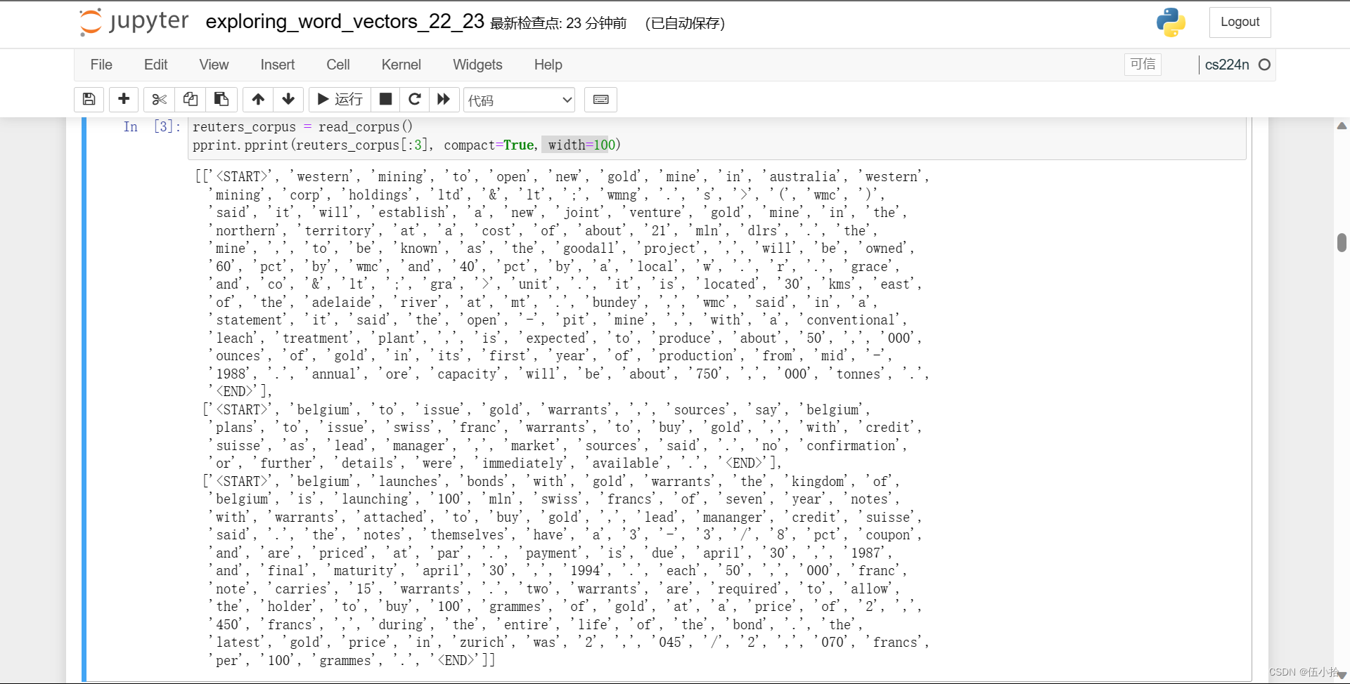
然后执行以下代码

 reuters_corpus = read_corpus()
 pprint.pprint(reuters_corpus[:3], compact=True, width=100)

会执行上面的read_corpus(category="gold")函数

然后把已处理的单词返回出来

Question 1.1: Implement distinct_words [code] (2 points)

题目

编写一个方法来计算语料库中出现的不同单词(单词类型)。你可以用for循环来做这件事，但用Python列表推导会更有效。特别地，这个链接可能有助于平面化列表的列表。如果你一般不熟悉Python列表推导式，这里有更多信息。

返回的' corpus_words '应该排序。你可以使用python的sorted函数。

你可能会发现使用Python sets删除重复的单词很有用。

代码

不管三七二十一, 先贴代码堵嘴总没错

 def distinct_words(corpus):
     """ Determine a list of distinct words for the corpus.
         Params:
             corpus (list of list of strings): corpus of documents
         Return:
             corpus_words (list of strings): sorted list of distinct words across the corpus
             n_corpus_words (integer): number of distinct words across the corpus
     """
     corpus_words = []
     n_corpus_words = -1
     
     ### SOLUTION BEGIN
     corpus_words=sorted(list(set([j for i in corpus for j in i])))
     n_corpus_words = len(corpus_words)
 ​
     ### SOLUTION END
 ​
     return corpus_words, n_corpus_words

以下是解释

Params:

• corpus: 就是之前返回的二重数组,

Return:

• corpus_words: 字符串数组

• n_corpus_words: corpus_words中元素个数

n_corpus_words很好实现, 直接用len

这里j for i in corpus for j in i建议参考上面的链接食用

先将二重数组降成一重的, 再set变成集合, 再list, 最后排序

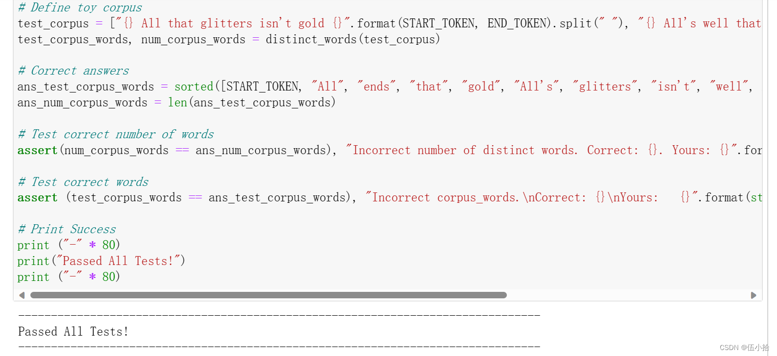
最后结果

Question 1.2: Implement compute_co_occurrence_matrix [code] (3 points)

编写一个方法，构造一个特定窗口大小的共现矩阵𝑛(默认值为4)，窗口的范围包括中间单词的前面n个单词和后面n个单词

在这里，我们开始使用numpy (np)来表示向量、矩阵和张量。如果你不熟悉NumPy，在本cs231n Python NumPy教程的后半部分有一个NumPy教程。

 def compute_co_occurrence_matrix(corpus, window_size=4):
     """ Compute co-occurrence matrix for the given corpus and window_size (default of 4).
     
         Note: Each word in a document should be at the center of a window. Words near edges will have a smaller
               number of co-occurring words.
               
               For example, if we take the document "<START> All that glitters is not gold <END>" with window size of 4,
               "All" will co-occur with "<START>", "that", "glitters", "is", and "not".
     
         Params:
             corpus (list of list of strings): corpus of documents
             window_size (int): size of context window
         Return:
             M (a symmetric numpy matrix of shape (number of unique words in the corpus , number of unique words in the corpus)): 
                 Co-occurence matrix of word counts. 
                 The ordering of the words in the rows/columns should be the same as the ordering of the words given by the distinct_words function.
             word2ind (dict): dictionary that maps word to index (i.e. row/column number) for matrix M.
     """
     words, n_words = distinct_words(corpus)
     M = None
     word2ind = {}
     
     ### SOLUTION BEGIN
     
     # 创建数组
     M = np.zeros((n_words,n_words))
     
     # 生成索引字典
     word2ind = {c:i for i,c in enumerate(words)}
     
     # 获得corpus里的单条语料
     for doc in corpus:
         total = len(doc)
         # print(doc)
         
     # 对单条doc中的所有单词进行循环, 依次作为中心词寻找两边的单词
         for i in range(len(doc)):
             center_word = doc[i]
             
             # 找出窗口内的所有单词
             start_index = (i-window_size) if (i-window_size>0) else 0
             end_index = (i+window_size) if (i+window_size<=total) else total
             window_words = doc[start_index:i] + doc[i+1:end_index+1]
             
             
             # 填写共现矩阵
             # 根据之前的索引字典找到单词对应的位置
             # 这里要求是一个对称矩阵, 但是不用在相反的位置再 +1, 共现矩阵本身就是对称的( 可以看上面那个矩阵自己比划一下)
             for w in window_words:
                 M[word2ind[center_word]][word2ind[w]] += 1
     ### SOLUTION END
 ​
     return M, word2ind

以下是解释

Params:

• corpus: 二维数组, 里面是字符串(语料)

• window_size: 窗口大小, 默认值是4

Return:

• M: 共现矩阵, 行/列中单词的顺序应该与distinct_words函数给出的单词顺序相同。

• word2ind: 字典, 将单词映射到矩阵M的索引(即行/列号)

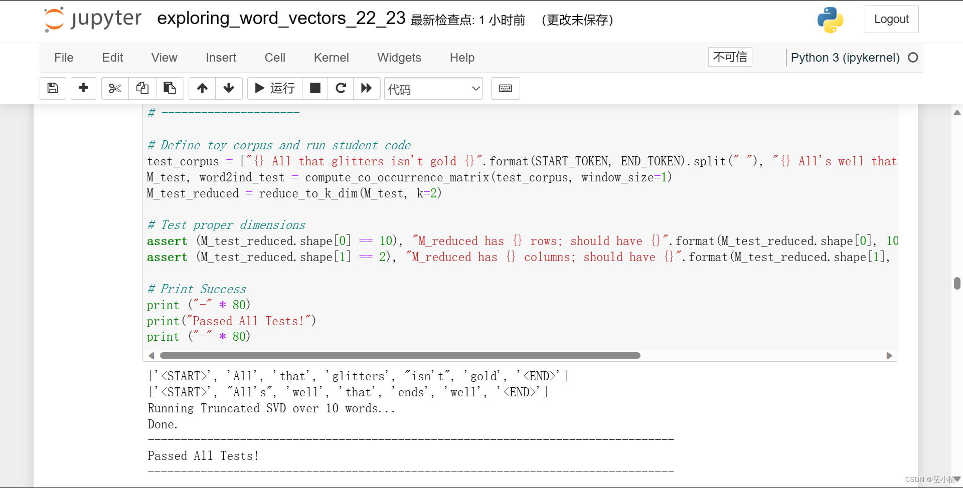
最后结果

Question 1.3: Implement reduce_to_k_dim [code] (1 point)

构造一种在矩阵上执行降维以产生k维嵌入的方法。使用奇异值分解(SVD)取最上面的k个分量，并产生一个新的k维嵌入矩阵。

注意:所有的numpy, scipy和scikit-learn ('sklearn)都提供了SVD的一些实现，但只有scipy和sklearn提供了截断SVD的实现，并且只有sklearn提供了计算大规模截断SVD的有效随机算法。所以请使用sklearn.decomposition.TruncatedSVD。

 def reduce_to_k_dim(M, k=2):
     """ Reduce a co-occurence count matrix of dimensionality (num_corpus_words, num_corpus_words)
         to a matrix of dimensionality (num_corpus_words, k) using the following SVD function from Scikit-Learn:
             - http://scikit-learn.org/stable/modules/generated/sklearn.decomposition.TruncatedSVD.html
     
         Params:
             M (numpy matrix of shape (number of unique words in the corpus , number of unique words in the corpus)): co-occurence matrix of word counts
             k (int): embedding size of each word after dimension reduction
         Return:
             M_reduced (numpy matrix of shape (number of corpus words, k)): matrix of k-dimensioal word embeddings.
                     In terms of the SVD from math class, this actually returns U * S
     """    
     n_iters = 10     # Use this parameter in your call to `TruncatedSVD`
     M_reduced = None
     print("Running Truncated SVD over %i words..." % (M.shape[0]))
     
     ### SOLUTION BEGIN
     
     # 创建降维后的矩阵 
     M_reduced = np.zeros((M.shape[0],k))
     
     # TruncatedSVD 方法的完整版
     # class sklearn.decomposition.TruncatedSVD(n_components=2, *, algorithm='randomized', n_iter=5, n_oversamples=10, power_iteration_normalizer='auto', random_state=None, tol=0.0)
     svd = TruncatedSVD(n_components = k, n_iter = n_iters)
     
     # 其实是两步, 第一步是fit来拟合这个变换, 然后再来transform将其应用于原始矩阵
     M_reduced = svd.fit_transform(M)
     ### SOLUTION END
 ​
     print("Done.")
     return M_reduced

以下是一些解释

Params:

• M: 共现矩阵(维度为语料中不重复单词数目 * 语料中不重复单词数目)

• k: 维度裁剪后每个 word 的嵌入维数

Return:

• M_reduced: SVD Decomposition 并裁剪之后的单词向量矩阵，维度为语料中不重复单词数目 * k

  (实际上是SVD变换中的 U * S 也就是左半拉部分)

关于TruncatedSVD

Dimensionality reduction using truncated SVD (aka LSA).

Parameters:

• n_components*int, default=2*

  Desired dimensionality of output data. If algorithm=’arpack’, must be strictly less than the number of features. If algorithm=’randomized’, must be less than or equal to the number of features. The default value is useful for visualisation. For LSA, a value of 100 is recommended.

• algorithm*{‘arpack’, ‘randomized’}, default=’randomized’*

  SVD solver to use. Either “arpack” for the ARPACK wrapper in SciPy (scipy.sparse.linalg.svds), or “randomized” for the randomized algorithm due to Halko (2009).

• n_iter*int, default=5*

  Number of iterations for randomized SVD solver. Not used by ARPACK. The default is larger than the default in randomized_svd to handle sparse matrices that may have large slowly decaying spectrum.

• n_oversamples*int, default=10*

  Number of oversamples for randomized SVD solver. Not used by ARPACK. See randomized_svd for a complete description.New in version 1.1.

• power_iteration_normalizer*{‘auto’, ‘QR’, ‘LU’, ‘none’}, default=’auto’*

  Power iteration normalizer for randomized SVD solver. Not used by ARPACK. See randomized_svd for more details.New in version 1.1.

• random_state*int, RandomState instance or None, default=None*

  Used during randomized svd. Pass an int for reproducible results across multiple function calls. See Glossary.

• tol*float, default=0.0*

  Tolerance for ARPACK. 0 means machine precision. Ignored by randomized SVD solver.

Attributes:

• components_ndarray of shape (n_components, n_features)

  The right singular vectors of the input data.

• explained_variance_ndarray of shape (n_components,)

  The variance of the training samples transformed by a projection to each component.

• explained_variance_ratio_ndarray of shape (n_components,)

  Percentage of variance explained by each of the selected components.

• singular_values_ndarray of shape (n_components,)

  The singular values corresponding to each of the selected components. The singular values are equal to the 2-norms of the n_components variables in the lower-dimensional space.

• n_features_in_int

  Number of features seen during fit.New in version 0.24.

• feature_names_in_ndarray of shape (n_features_in_,)

  Names of features seen during fit. Defined only when X has feature names that are all strings.New in version 1.0.

关于fit_transform

关于fit_transform

fit_transform(X, y=None)[source]

Fit model to X and perform dimensionality reduction on X.

• Parameters:

  X*{array-like, sparse matrix} of shape (n_samples, n_features)Training data.yIgnored*Not used, present here for API consistency by convention.

• Returns:

  X_new*ndarray of shape (n_samples, n_components)*Reduced version of X. This will always be a dense array.

最后结果

Question 1.4: Implement plot_embeddings [code] (1 point)¶

在这里，你将编写一个函数来在二维空间中绘制一组二维向量。对于图形，我们将使用Matplotlib (plt)。

对于本例，您可能会发现调整此代码很有用。将来，制作图表的一个好方法是查看Matplotlib图库，找到一个看起来有点像您想要的图表，并调整它们提供的代码。

 def plot_embeddings(M_reduced, word2ind, words):
     """ Plot in a scatterplot the embeddings of the words specified in the list "words".
         NOTE: do not plot all the words listed in M_reduced / word2ind.
         Include a label next to each point.
         
         Params:
             M_reduced (numpy matrix of shape (number of unique words in the corpus , 2)): matrix of 2-dimensioal word embeddings
             word2ind (dict): dictionary that maps word to indices for matrix M
             words (list of strings): words whose embeddings we want to visualize
     """
 ​
     ### SOLUTION BEGIN
     for w in words: 
         x = M_reduced[word2ind[w]][0]
         y = M_reduced[word2ind[w]][1]
         plt.scatter(x,y, marker='x', color='blue')
         plt.text(x, y, w, fontsize=9)
     plt.show()
     ### SOLUTION END

Params:

• M_reduced: SVD降维处理后的单词嵌入矩阵

• word2ind: 从单词到M下标的映射关系

• words: 需要嵌入然后绘制的单词lest

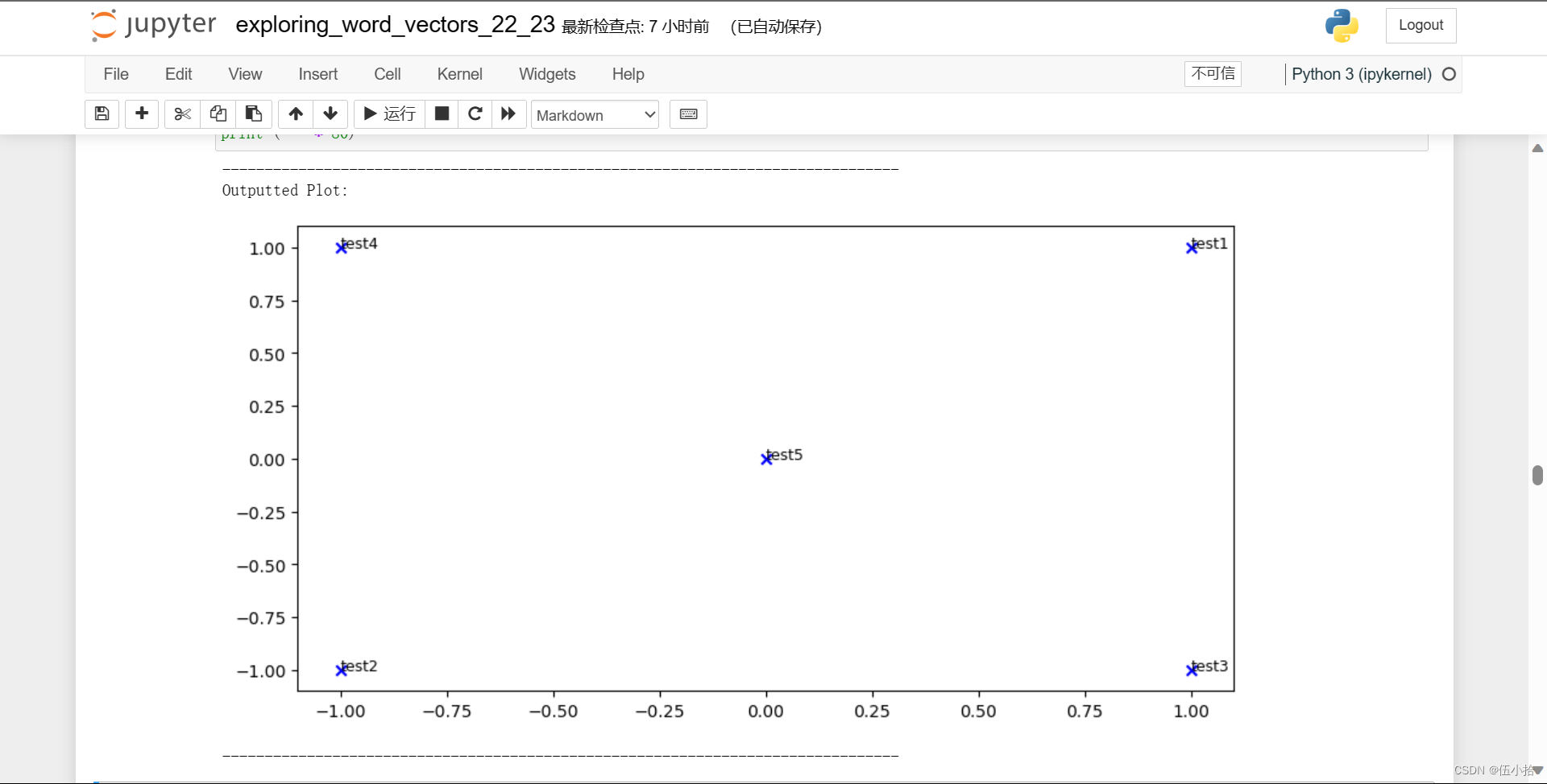
最后结果

Question 1.5: Co-Occurrence Plot Analysis [written] (3 points)

现在我们将把你写的所有部分组合起来! 我们将在路透社“gold”语料库上计算具有固定窗口4(默认窗口大小)的共现矩阵。然后我们将使用TruncatedSVD来计算每个单词的二维嵌入。TruncatedSVD返回U*S，所以我们需要规范化返回的向量，这样所有的向量都将出现在单位圆周围(因此亲密度是方向亲密度)。

注:下面进行规范化的代码行使用了NumPy的“广播”概念。如果你不知道广播，请查看数组上的计算:广播由Jake VanderPlas。

运行下面的单元格生成图表。可能需要几秒钟才能运行。

代码我就不贴了, 直接放图片

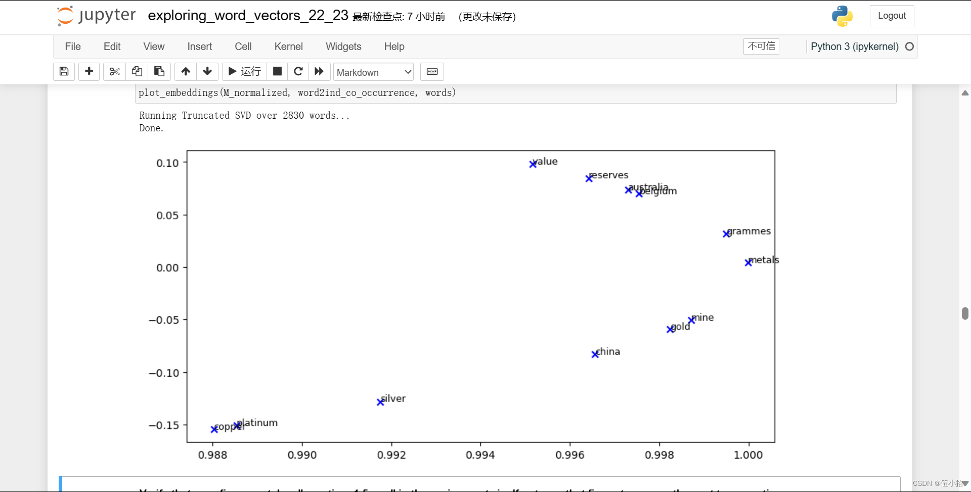
这是代码生成的, 在压缩包里还有一个标准图片

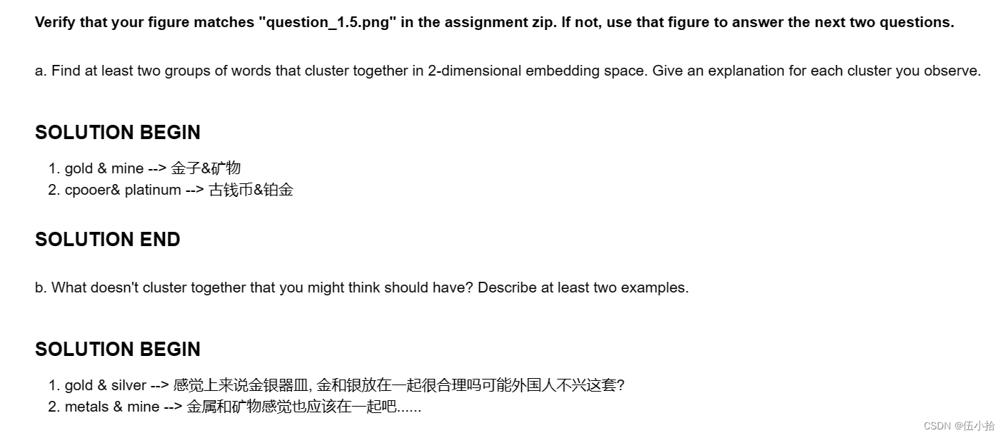
验证你的图形是否与压缩文件中的“question_1.5.png”匹配。如果不是，用这个图片来回答接下来的两个问题。

a.在二维嵌入空间中找到至少两组聚类在一起的词。对你观察到的每一个群集作出解释。

b.哪些你认为应该聚在一起却没有聚在一起的东西?描述至少两个例子。

我直接贴截图了

Part 2: Prediction-Based Word Vectors (15 points)

正如在课堂上所讨论的，最近基于预测的词向量表现出了更好的性能，例如word2vec和GloVe(它也利用了计数的好处)。在这里，我们将探索GloVe生产的嵌入。有关word2vec和GloVe算法的更多细节，请参阅课堂笔记和讲座幻灯片。如果你想冒险，挑战一下自己，试着阅读GloVe的原始论文。

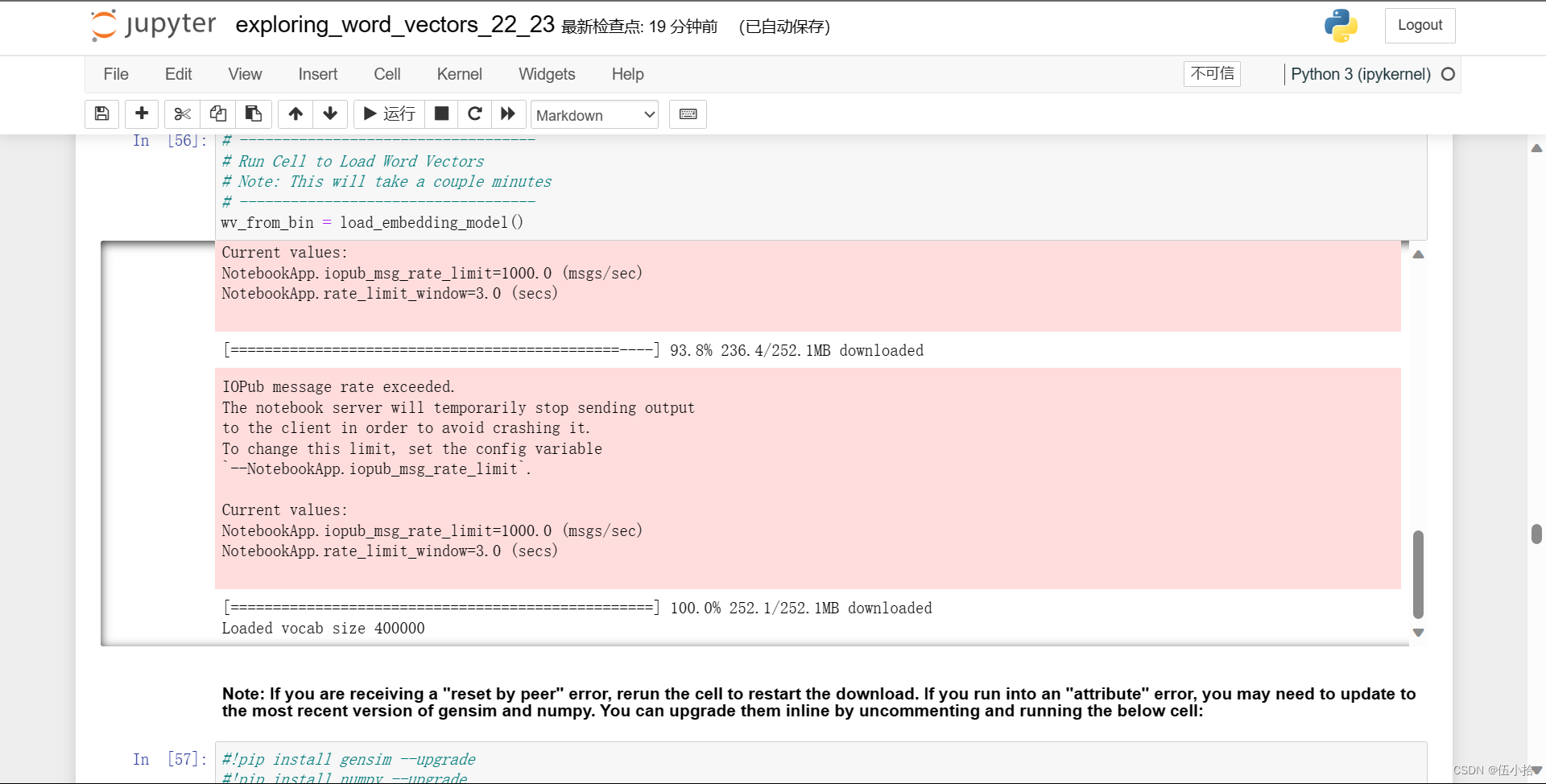
然后运行以下单元，将GloVe矢量加载到内存中。注意:如果这是您第一次运行这些单元格，即下载嵌入模型，则需要几分钟才能运行。如果您以前运行过这些单元格，重新运行它们将加载模型而无需重新下载，这将花费大约1到2分钟。

Note: If you are receiving a "reset by peer" error, rerun the cell to restart the download. If you run into an "attribute" error, you may need to update to the most recent version of gensim and numpy. You can upgrade them inline by uncommenting and running the below cell:

下载结果:这里粉色不是报错

Reducing dimensionality of Word Embeddings

让我们直接将GloVe嵌入与共生矩阵的嵌入进行比较。为了避免内存耗尽，我们将使用10000个GloVe向量的样本。

1. 将10000个 Glove 向量放入矩阵M中

2. 运行reduce_to_k_dim(之前写的 Truncated SVD 函数)将向量从200维减少到2维。

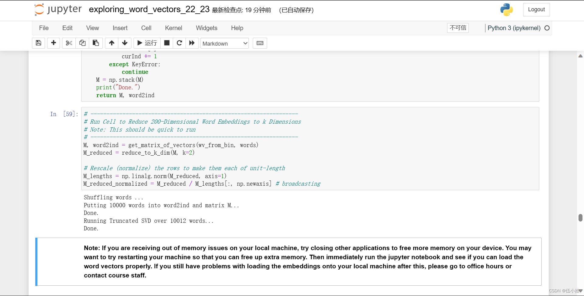
Note: If you are receiving out of memory issues on your local machine, try closing other applications to free more memory on your device. You may want to try restarting your machine so that you can free up extra memory. Then immediately run the jupyter notebook and see if you can load the word vectors properly. If you still have problems with loading the embeddings onto your local machine after this, please go to office hours or contact course staff.

Question 2.1: GloVe Plot Analysis [written] (3 points)¶

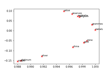
运行下面的单元格，绘制['value', 'gold', 'platinum', 'reserves', 'silver', 'metals', 'copper', 'belgium', 'australia', 'china', 'grammes', "mine"]的2D GloVe嵌入图。

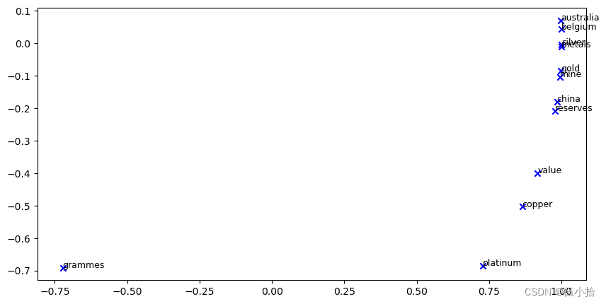
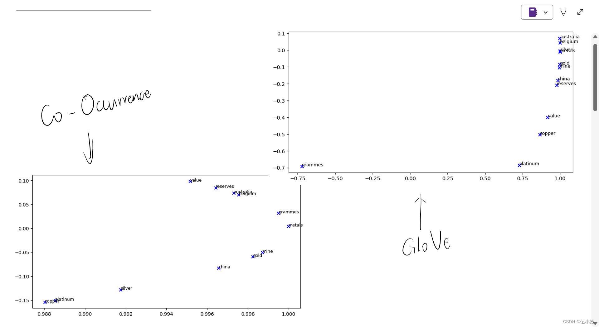
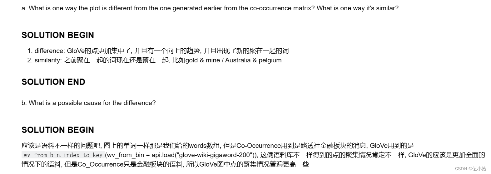
a.该图与之前由共现矩阵生成的图有什么不同?有什么相似之处?

b.造成差异的可能原因是什么?

这里先将两个图放在一起方便对比

我直接放解释了

Cosine Similarity

现在我们有了单词向量，我们需要一种方法来量化单个单词之间的相似性，根据这些向量。其中一个度量就是余弦相似度。我们将用它来查找彼此“近”和“远”的单词。

我们可以把n维向量看作n维空间中的点。如果我们从这个角度来看L1和L2，距离有助于量化两点之间“我们必须旅行”的空间量。另一种方法是检查两个向量之间的夹角。从三角学中我们知道:

不计算实际角度，我们可以用similarity = cos(\Theta)表示相似度。形式上，两个向量p和q之间的余弦相似度 s定义为:

$$
s = \frac{p \cdot q}{||p|| ||q||}, \textrm{ where } s \in [-1, 1]
$$

Question 2.2: Words with Multiple Meanings (1.5 points) [code + written]

Polysemes and homonyms are words that have more than one meaning (see this wiki page to learn more about the difference between polysemes and homonyms ).

Find a word with at least two different meanings such that the top-10 most similar words (according to cosine similarity) contain related words from both meanings.

For example, "leaves" has both "go_away" and "a_structure_of_a_plant" meaning in the top 10, and "scoop" has both "handed_waffle_cone" and "lowdown". You will probably need to try several polysemous or homonymic words before you find one.

多义词和同音异义词是指有多个意思的词(参见这个维基页面了解更多关于多义词和同音异义词的区别)。找到一个有“至少两个不同意思”的单词，使前10个最相似的单词(根据余弦相似度)包含“两个”意思的相关单词。例如，“leaves”在余弦相似度前10名中有“离开”和“植物某部分结构”的意思，“scoop”有“手拿的华夫蛋筒(?)”和“真相内幕”的意思。在找到一个词之前，你可能需要尝试几个多义词或同音词。

请说出你发现的单词以及出现在前10名中的多个含义。为什么你认为你尝试过的许多多义词或同音词都不起作用(即最相似的10个词只包含单词的一个的意思)?

注意:您应该使用' wv_from_bin.most_similar(word) '函数来获取前10个相似的单词。这个函数根据与给定单词的余弦相似度对词汇表中所有其他单词进行排序。如需进一步帮助，请查看GenSim文档)。

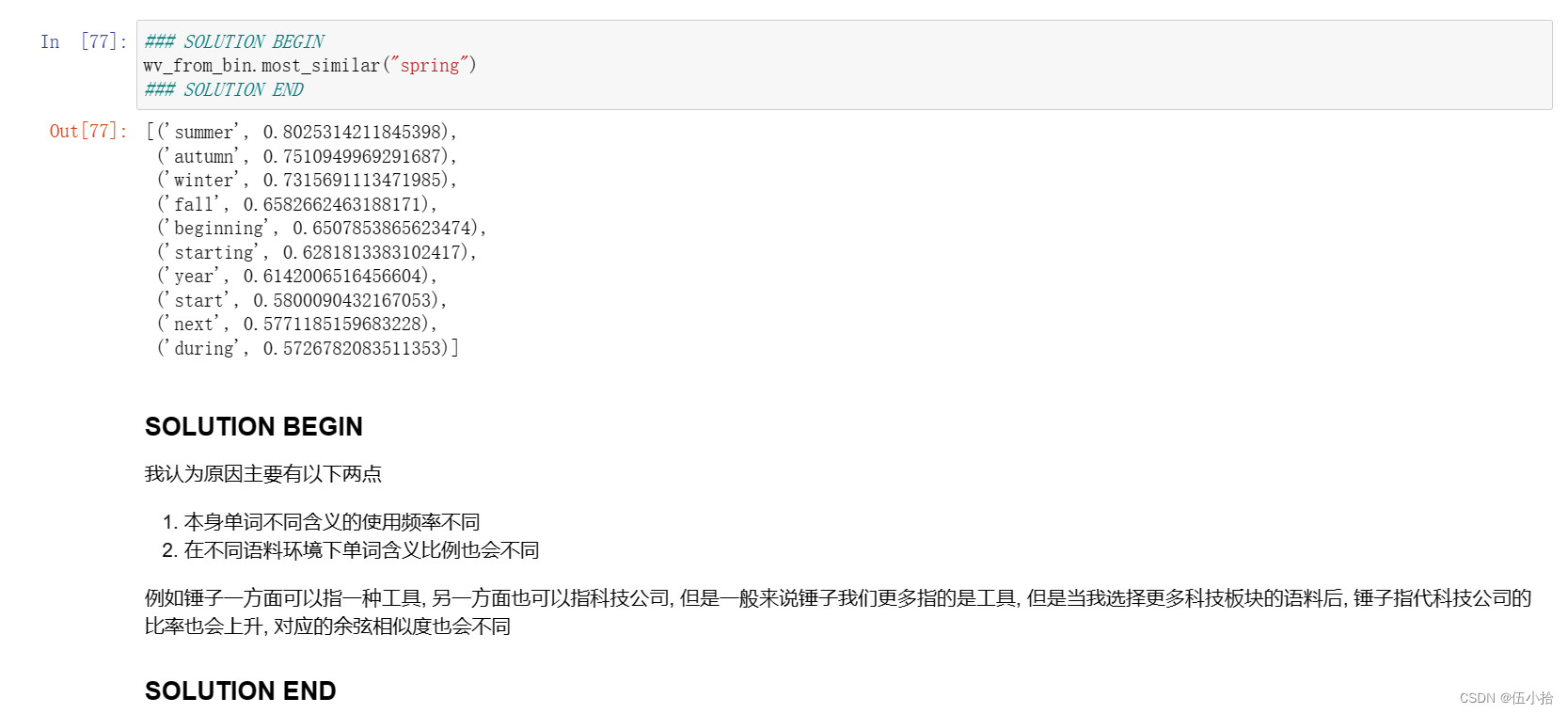
含义我就不说了, 直接上截图吧

这里spring是作为只有一个含义的例子

Question 2.3: Synonyms & Antonyms (2 points) [code + written]

当考虑余弦相似度时，考虑余弦距离通常更方便，它等于1 -余弦相似度。

找三个词(𝑤1，𝑤2，𝑤3), 在𝑤1和𝑤2是同义词和𝑤1和𝑤3是反义词的情况下，余弦距离(𝑤1，𝑤3)<余弦距离(𝑤1，𝑤2)

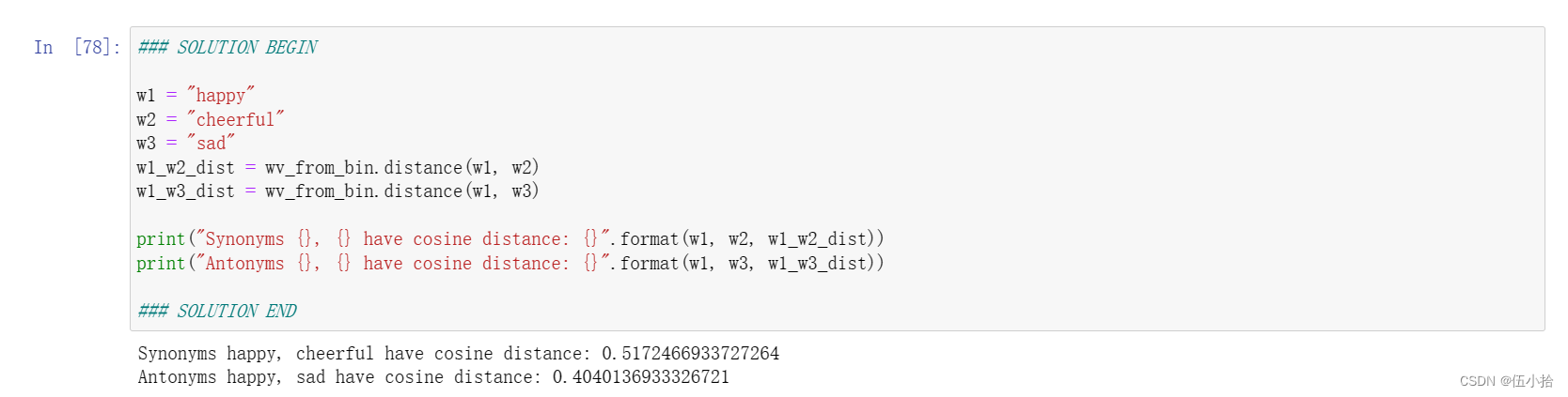
例如与𝑤2 = "快乐"相比𝑤1 = “happy”更接近𝑤3 =“悲伤”。请找一个满足上述条件的不同例子。一旦你找到了你的例子，请给出一个可能的解释，为什么这种反直觉的结果可能会发生。

您应该使用wv_from_bin。Distance (w1, w2)函数来计算两个词之间的余弦距离。请参阅GenSim文档以获得进一步帮助。

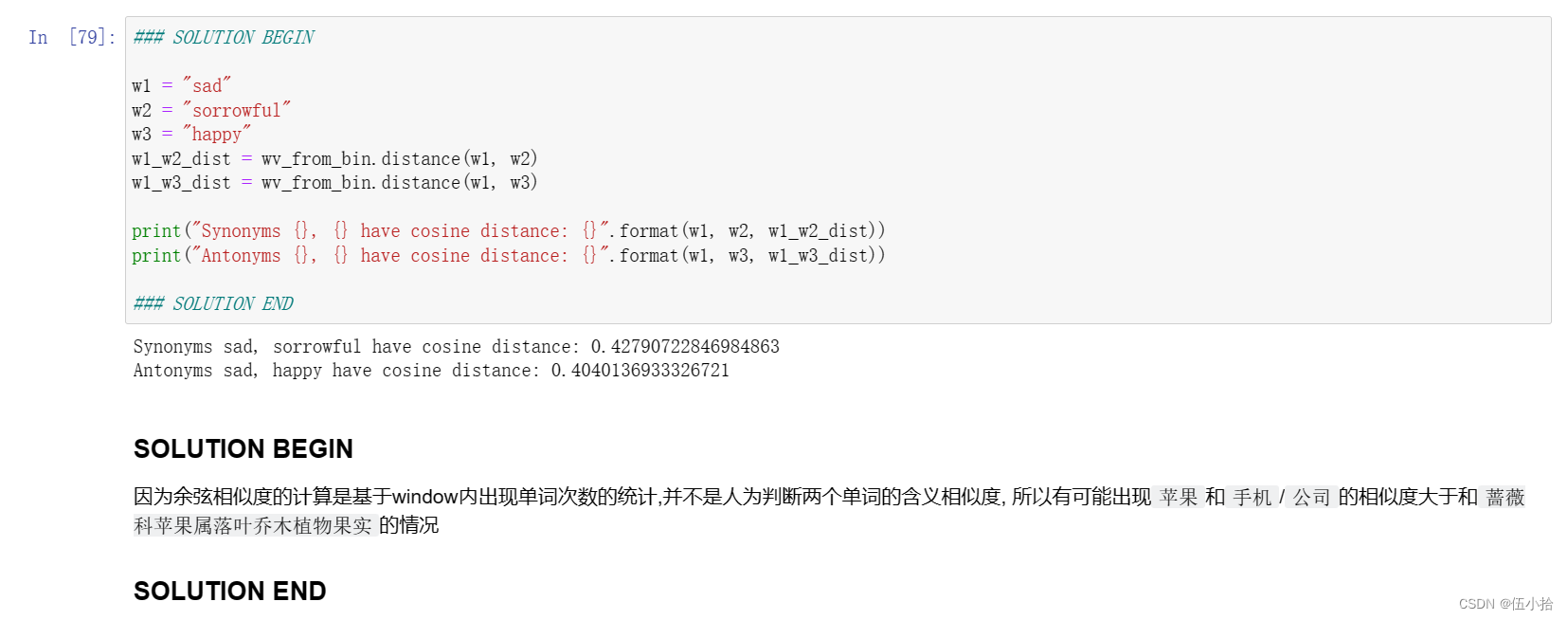
先验证上面的例子, 反过来换个反义词就是我的了

Question 2.4: Analogies with Word Vectors [written] (1.5 points)

单词向量已被证明“有时”表现出解决类比的能力。

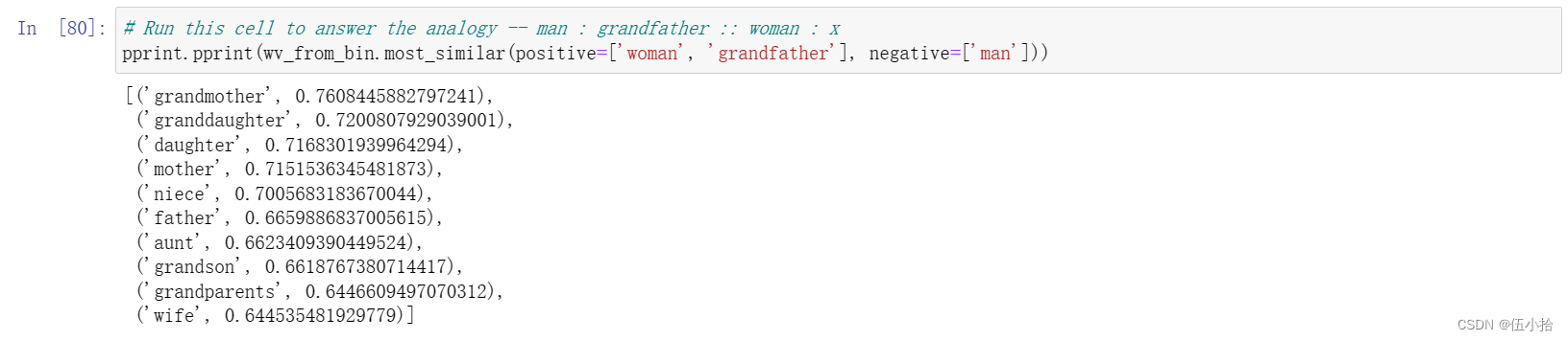
举个例子，对于类比“男人:祖父::女人:x”(读作:男人之于祖父就像女人之于x)， x是什么?

在下面的单元格中，我们将向您展示如何使用GenSim文档中的most_similar函数来使用单词向量查找x )。该函数查找与“正面”列表中最相似的单词，以及与“负面”列表中最不相似的单词(同时省略通常最相似的输入单词;参见本文)。类比的答案将具有最高的余弦相似性(返回的最大数值)。

In the cell below, we show you how to use word vectors to find x using the most_similar function from the GenSim documentation. The function finds words that are most similar to the words in the positive list and most dissimilar from the words in the negative list (while omitting the input words, which are often the most similar; see this paper). The answer to the analogy will have the highest cosine similarity (largest returned numerical value).

这里放一下运行结果

让𝑚,𝑔,𝑤以及x分别表示男人、祖父、女人和答案的单词向量。只使用矢量𝑚,𝑔,𝑤，以及向量算术运算符+和−在你的答案中，我们最大化的是哪个表达式余弦相似度?

提示:回想一下，单词向量只是表示单词的多维向量。使用每个向量的任意位置绘制一个2D示例可能会有所帮助。男人和女人在相对于祖父的坐标平面上的位置和答案是什么?

$$
\frac{(g-m+w) x }{|g-m+w|}
$$

Question 2.5: Finding Analogies [code + written] (1.5 points)

a.对于前面的例子，很明显，“祖母”完成了这个类比。但是，请直观地解释一下，为什么“最相似”函数会给我们“孙女”、“女儿”或“母亲”这样的词?

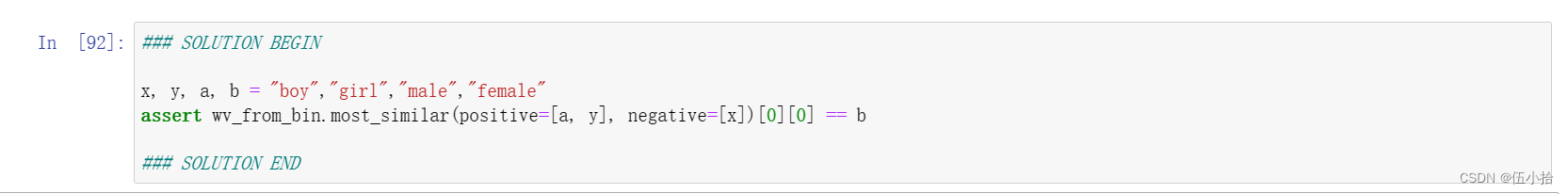
b.根据这些向量找到一个类比的例子(即预期的单词排在最前面)。在你的解决方案中，请以x:y:: a:b的形式陈述完整的类比。如果你认为这个类比很复杂，用一到两句话解释为什么这个类比成立。

注意:你可能需要尝试许多类比来找到一个有效的!

a.

因为这里从男人到祖父不仅可以指的是祖辈, 还可以有更广泛的亲缘关系的含义, 在这种情况下, 孙女女儿之类的都符合条件

b.

本来想换换的, 但是懒得一个个试过去了, 所以照葫芦画瓢换了一个

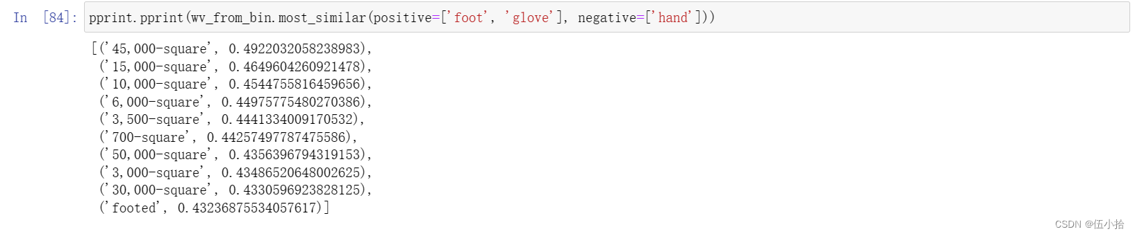
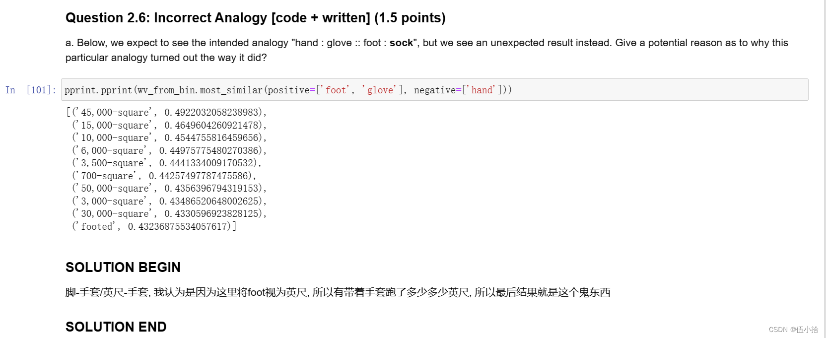
Question 2.6: Incorrect Analogy [code + written] (1.5 points)

a.在下面，我们期望看到预期的类比“手:手套::脚:袜子”，但是我们看到了一个意想不到的结果。给出一个可能的原因，为什么这个特殊的类比会变成这样?

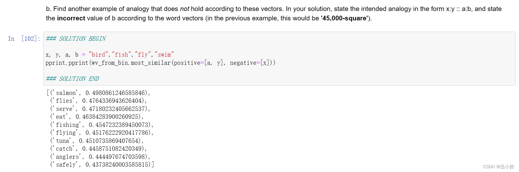
b.根据这些向量找到另一个不成立的类比例子。在您的解决方案中，以x:y:: a:b的形式陈述预期的类比，并根据单词向量陈述不正确的值(在前面的示例中，这将是'45,000平方')。

累了, 我为什么要解释这个

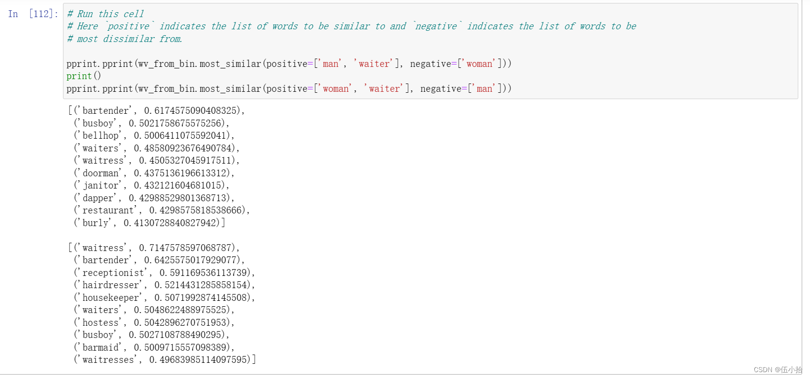
Question 2.7: Guided Analysis of Bias in Word Vectors [written] (1 point)

认识到我们的词嵌入中隐含的偏见(性别、种族、性取向等)是很重要的。偏见可能是危险的，因为它可以通过使用这些模型的应用程序强化刻板印象。

运行下面的单元格，检查(a)哪些术语与“女人”和“职业”最相似，与“男人”最不相似，以及(b)哪些术语与“男人”和“职业”最相似，与“女人”最不相似。指出女性相关词汇和男性相关词汇的区别，并解释它是如何反映性别偏见的。

啧, 不想解释了, 反正呈现出来就是这样

Question 2.8: Independent Analysis of Bias in Word Vectors [code + written] (1 point)

使用most_similar函数找到另一对类比，表明向量表现出一些偏差。请简单解释一下你发现的偏见的例子。

不想找了, 累了

Question 2.9: Thinking About Bias [written] (2 points)

a.给出一个解释，说明偏见是如何进入词向量的。简要描述一个真实世界的例子来证明这种偏见的来源。

b.你可以用什么方法来减轻词向量所表现出的偏见?简要描述一个演示此方法的实际示例。

语料库选择上的偏见会导致词向量表现出的不一致, 方法就是扩大语料库

终于写完了, 撒花

最后放个猫猫

这是封面小猫, 它叫Chip, 喜欢凉凉的铝板

小猫可爱捏~