# 导入所需的库
import pandas as pd # 导入pandas库,用于数据处理和分析,特别是DataFrame操作
import numpy as np # 导入numpy库,用于进行数值计算,特别是数组操作
import matplotlib.pyplot as plt # 导入matplotlib的pyplot模块,用于绘制图表
import matplotlib # 导入matplotlib主库,用于更底层的绘图设置
from matplotlib.patches import Patch # 从matplotlib.patches中导入Patch,用于创建图例中的色块
from sklearn.model_selection import train_test_split, GridSearchCV # 从sklearn导入数据划分和网格搜索交叉验证的工具
from sklearn.preprocessing import StandardScaler # 从sklearn导入数据标准化工具
import xgboost as xgb # 【XGBoost 修改】导入XGBoost库,用于构建梯度提升决策树模型
from sklearn.metrics import mean_absolute_error, r2_score, mean_squared_error # 从sklearn导入评估回归模型性能的指标
import joblib # 导入joblib库,用于模型的保存和加载
from scipy.stats import gaussian_kde # 从scipy.stats导入高斯核密度估计,可用于绘制密度图(此脚本中未直接使用,但可能为备用)
from sklearn.inspection import PartialDependenceDisplay, partial_dependence # 从sklearn导入部分依赖图的工具(此脚本未使用,改用手动实现)
import time # 导入time库,用于计时(此脚本中未直接使用)
import os # 导入os库,用于操作系统相关功能,如创建文件夹
from itertools import combinations # 从itertools导入combinations,用于生成组合
import shap # 导入shap库,用于模型解释,计算SHAP值
import warnings # 导入warnings库,用于控制警告信息的显示
from collections import defaultdict # 从collections导入defaultdict,用于创建带有默认值的字典
from PyALE import ale # 导入PyALE库,用于计算和绘制累积局部效应图
from scipy.interpolate import griddata # 从scipy.interpolate导入griddata,用于插值(此脚本中未直接使用)
# --- 全局设置 ---
# 忽略特定类型的警告,避免在输出中显示不必要的警告信息
warnings.filterwarnings("ignore", category=FutureWarning, module="sklearn.utils._bunch")
warnings.filterwarnings("ignore", category=UserWarning)
matplotlib.use('TkAgg') # 设置matplotlib的后端,'TkAgg'是一个图形界面后端,确保在某些环境下可以正常显示绘图窗口
import os
import tempfile
# 设置临时文件夹到一个英文路径
os.environ['JOBLIB_TEMP_FOLDER'] = 'C:/temp'
os.environ['TMP'] = 'C:/temp'
os.environ['TEMP'] = 'C:/temp'
# 确保这个目录存在
if not os.path.exists('C:/temp'):
os.makedirs('C:/temp')
# --- (函数定义区) ---
# 定义一个函数,用于绘制回归模型的拟合效果图
def plot_regression_fit(y_true, y_pred, r2, rmse, mae, data_label_en, title_en, save_path):
"""
绘制真实值与预测值的散点图,并显示模型评估指标。
y_true: 真实值
y_pred: 预测值
r2: R-squared值
rmse: 均方根误差
mae: 平均绝对误差
data_label_en: 数据集标签 (如 'Train Set')
title_en: 图表标题
save_path: 图片保存路径
"""
plt.style.use('seaborn-v0_8-whitegrid') # 使用预设的绘图风格
plt.rcParams['font.family'] = 'sans-serif' # 设置字体为无衬线字体,以获得更好的显示效果
fig, ax = plt.subplots(figsize=(7, 7)) # 创建一个7x7英寸的画布和子图
# 绘制真实值 vs 预测值的散点图
ax.scatter(y_true, y_pred, alpha=0.6, edgecolors='k', label=f'{data_label_en} (n={len(y_true)})')
# 计算并设置坐标轴的范围,确保1:1线能完整显示
lims = [np.min([y_true.min(), y_pred.min()]) - 5, np.max([y_true.max(), y_pred.max()]) + 5]
# 绘制1:1参考线 (y=x),代表完美预测
ax.plot(lims, lims, 'k--', alpha=0.75, zorder=0, label='1:1 Line (Perfect Fit)')
ax.set_aspect('equal') # 设置x和y轴的比例相等
ax.set_xlim(lims) # 设置x轴范围
ax.set_ylim(lims) # 设置y轴范围
y_true_np = np.array(y_true) # 将真实值转换为numpy数组
y_pred_np = np.array(y_pred) # 将预测值转换为numpy数组
m, b = np.polyfit(y_true_np, y_pred_np, 1) # 对散点进行线性拟合,得到斜率m和截距b
ax.plot(y_true_np, m * y_true_np + b, 'r-', label='Linear Fit') # 绘制线性拟合线
ax.set_xlabel('True Values (%)', fontsize=12) # 设置x轴标签
ax.set_ylabel('Predicted Values (%)', fontsize=12) # 设置y轴标签
ax.set_title(title_en, fontsize=14, weight='bold') # 设置图表标题
# 准备要在图上显示的评估指标文本
metrics_text = f'$R^2 = {r2:.3f}$\n$RMSE = {rmse:.3f}$\n$MAE = {mae:.3f}$'
# 在图的左上角添加文本框,显示评估指标
ax.text(0.05, 0.95, metrics_text, transform=ax.transAxes, fontsize=12, verticalalignment='top',
bbox=dict(boxstyle='round', facecolor='wheat', alpha=0.5))
ax.legend(loc='lower right') # 在右下角显示图例
fig.savefig(save_path, dpi=200, bbox_inches='tight') # 保存图表到指定路径
plt.close(fig) # 关闭图表,释放内存
# 定义一个函数,用于绘制组合特征重要性图(条形图+甜甜圈图)
def plot_importance_combined(df_importance, title, save_path, bar_color='dodgerblue'):
"""
绘制特征重要性条形图,并在右下角嵌入一个显示Top-N特征占比的甜甜圈图。
df_importance: 包含'Feature'和'Importance'两列的DataFrame
title: 图表标题
save_path: 图片保存路径
bar_color: 条形图的颜色
"""
df_importance_sorted = df_importance.sort_values(by='Importance', ascending=True) # 按重要性升序排序
plt.rc("font", family='Microsoft YaHei') # 设置中文字体为微软雅黑,以正确显示中文
fig, ax = plt.subplots(figsize=(14, 10)) # 创建一个14x10英寸的画布和子图
# 绘制水平条形图
bars = ax.barh(df_importance_sorted['Feature'], df_importance_sorted['Importance'], color=bar_color, alpha=0.8)
ax.set_title(title, fontsize=18, pad=20) # 设置标题
ax.set_xlabel('重要性得分', fontsize=14) # 设置x轴标签
ax.set_ylabel('特征', fontsize=14) # 设置y轴标签
ax.tick_params(axis='both', which='major', labelsize=12) # 设置刻度标签的大小
ax.grid(axis='x', linestyle='--', alpha=0.6) # 显示x轴方向的网格线
# 在每个条形图旁边显示具体的重要性数值
for bar in bars:
width = bar.get_width()
ax.text(width, bar.get_y() + bar.get_height() / 2,
f' {width:.4f}', va='center', ha='left', fontsize=10)
ax.set_xlim(right=ax.get_xlim()[1] * 1.2) # 调整x轴范围,为数值标签留出空间
N_DONUT_FEATURES = 5 # 设置甜甜圈图中要显示的特征数量
if len(df_importance) < N_DONUT_FEATURES: # 如果总特征数小于5,则取全部特征
N_DONUT_FEATURES = len(df_importance)
df_desc = df_importance.sort_values(by='Importance', ascending=False) # 按重要性降序排序
top_n_features = df_desc.head(N_DONUT_FEATURES) # 选取最重要的N个特征
donut_feature_names = top_n_features['Feature'].tolist() # 获取这N个特征的名称
# 如果有特征且总重要性大于0,则绘制甜甜圈图
if not top_n_features.empty and top_n_features['Importance'].sum() > 0:
total_donut_importance = top_n_features['Importance'].sum() # 计算Top-N特征的重要性总和
donut_percentages = top_n_features['Importance'] / total_donut_importance * 100 # 计算每个特征在Top-N中的百分比
ax_inset = fig.add_axes([0.45, 0.15, 0.28, 0.28]) # 在主图上创建一个嵌入的子图(甜甜圈图的位置)
colors = matplotlib.colormaps['tab10'].colors # 获取一组颜色
# 绘制饼图(通过设置width属性使其变为甜甜圈图)
wedges, _ = ax_inset.pie(
donut_percentages,
colors=colors[:len(top_n_features)], startangle=90, counterclock=False,
wedgeprops=dict(width=0.45, edgecolor='w')
)
# 计算Top-N特征占总特征重要性的比例
subset_importance_ratio = top_n_features['Importance'].sum() / df_importance['Importance'].sum()
# 在甜甜圈中心添加文本
ax_inset.text(0, 0, f'Top {N_DONUT_FEATURES} 特征\n占总重要性\n{subset_importance_ratio:.2%}',
ha='center', va='center', fontsize=9, linespacing=1.4)
label_threshold = 3.0 # 设置标签显示的阈值,小于此值的百分比会用引导线引出
y_text_offsets = {'left': 1.4, 'right': 1.4} # 初始化引导线标签的垂直偏移量
# 为每个扇区添加百分比标签
for i, p in enumerate(wedges):
percent = donut_percentages.iloc[i]
ang = (p.theta2 - p.theta1) / 2. + p.theta1 # 计算扇区中心角度
y = np.sin(np.deg2rad(ang)) # 计算标签的y坐标
x = np.cos(np.deg2rad(ang)) # 计算标签的x坐标
# 如果百分比小于阈值,使用引导线
if percent < label_threshold and percent > 0:
side = 'right' if x > 0 else 'left' # 判断标签在左侧还是右侧
y_pos = y_text_offsets[side] # 获取当前侧的y偏移
y_text_offsets[side] += -0.2 if y > 0 else 0.2 # 更新偏移量,避免标签重叠
connectionstyle = f"angle,angleA=0,angleB={ang}" # 设置引导线样式
# 添加带引导线的注释
ax_inset.annotate(f'{percent:.1f}%', xy=(x, y), xytext=(0.2 * np.sign(x), y_pos),
fontsize=9, ha='center',
arrowprops=dict(arrowstyle="-", connectionstyle=connectionstyle, relpos=(0.5, 0.5)))
# 如果百分比大于阈值,直接在扇区内显示
elif percent > 0:
ax_inset.text(x * 0.8, y * 0.8, f'{percent:.1f}%', ha='center', va='center', fontsize=9,
fontweight='bold', color='white')
# 在甜甜圈图右侧添加图例
ax_inset.legend(wedges, donut_feature_names,
loc="center left", bbox_to_anchor=(1.2, 0.5),
frameon=False, fontsize=11)
plt.savefig(save_path, dpi=720, bbox_inches='tight') # 保存高分辨率图表
plt.close(fig) # 关闭图表,释放内存
# 定义一个函数,用于绘制残差图
def plot_residuals_styled(residuals, y_pred, save_path, title):
"""
绘制残差与预测值的关系图,并高亮显示异常值。
residuals: 残差 (真实值 - 预测值)
y_pred: 预测值
save_path: 图片保存路径
title: 图表标题
"""
plt.style.use('seaborn-v0_8-whitegrid') # 使用预设绘图风格
plt.rc("font", family='Microsoft YaHei') # 设置中文字体
fig, ax = plt.subplots(figsize=(10, 8)) # 创建一个10x8英寸的画布
sd_residuals = np.std(residuals) # 计算残差的标准差
is_outlier = np.abs(residuals) > 2 * sd_residuals # 定义异常值:绝对残差大于2倍标准差
num_outliers = np.sum(is_outlier) # 计算异常值的数量
print(f"在数据集 '{title}' 中, 共找到 {num_outliers} 个异常值 (残差 > 2 S.D.)。") # 打印异常值信息
sd_label = f'S.D. (±{sd_residuals:.2f})' # 准备标准差区间的图例标签
ax.axhspan(-sd_residuals, sd_residuals, color='yellow', alpha=0.3, label=sd_label) # 绘制一个表示一个标准差范围的水平区域
# 绘制正常值的散点图
ax.scatter(y_pred[~is_outlier], residuals[~is_outlier], alpha=0.6, c='green', edgecolors='k', linewidth=0.5, s=50,
label='正常值')
# 绘制异常值的散点图
ax.scatter(y_pred[is_outlier], residuals[is_outlier], alpha=0.8, c='red', edgecolors='k', linewidth=0.5, s=70,
label='异常值 (> 2 S.D.)')
ax.axhline(0, color='black', linestyle='--', linewidth=1.5) # 绘制残差为0的参考线
ax.set_title(title, fontsize=16, weight='bold') # 设置标题
ax.set_xlabel('预测值', fontsize=14) # 设置x轴标签
ax.set_ylabel('残差 (真实值 - 预测值)', fontsize=14) # 设置y轴标签
# 设置图表边框样式
for spine in ax.spines.values():
spine.set_visible(True)
spine.set_color('black')
spine.set_linewidth(1)
ax.legend(loc='upper right', fontsize=12) # 显示图例
y_max = np.max(np.abs(residuals)) * 1.2 # 计算y轴的范围
ax.set_ylim(-y_max, y_max) # 设置y轴范围
plt.tight_layout() # 调整布局,防止标签重叠
plt.savefig(save_path, dpi=300, bbox_inches='tight') # 保存图表
plt.close() # 关闭图表
# =========================================================================
# ======================= 新增:手动PDP计算与绘图函数 =======================
# =========================================================================
def manual_pdp_1d(model, X_data, feature_name, grid_resolution=50):
"""
手动计算一维部分依赖(PDP)和个体条件期望(ICE)数据。
返回:
- grid_values: 特征的网格点。
- pdp_values: 对应的PDP值 (ICE的均值)。
- ice_lines: 所有样本的ICE线数据。
"""
# 在特征的最小值和最大值之间生成一系列网格点
grid_values = np.linspace(X_data[feature_name].min(), X_data[feature_name].max(), grid_resolution)
# 初始化一个数组来存储每个样本的ICE线数据
ice_lines = np.zeros((len(X_data), grid_resolution))
# 遍历数据集中每一个样本
for i, (_, sample) in enumerate(X_data.iterrows()):
# 创建一个临时DataFrame,行数为网格点数,内容为当前样本的重复
temp_df = pd.DataFrame([sample] * grid_resolution)
# 将要分析的特征列替换为网格值
temp_df[feature_name] = grid_values
# 使用模型进行预测,得到这个样本在不同特征值下的预测结果,即ICE线
ice_lines[i, :] = model.predict(temp_df)
# PDP是所有ICE线的平均值,在每个网格点上求均值
pdp_values = np.mean(ice_lines, axis=0)
# 返回计算结果
return grid_values, pdp_values, ice_lines
def manual_pdp_2d(model, X_data, features_tuple, grid_resolution=20):
"""
手动计算二维部分依赖(PDP)数据。
返回:
- grid_1: 第一个特征的网格点。
- grid_2: 第二个特征的网格点。
- pdp_values: 二维网格上对应的PDP值。
"""
feat1_name, feat2_name = features_tuple # 获取两个特征的名称
# 为第一个特征生成网格点
grid_1 = np.linspace(X_data[feat1_name].min(), X_data[feat1_name].max(), grid_resolution)
# 为第二个特征生成网格点
grid_2 = np.linspace(X_data[feat2_name].min(), X_data[feat2_name].max(), grid_resolution)
# 初始化一个二维数组来存储PDP值
pdp_values = np.zeros((grid_resolution, grid_resolution))
# 遍历二维网格的每一个点
for i, val1 in enumerate(grid_1):
for j, val2 in enumerate(grid_2):
# 创建一个原始数据的临时副本
X_temp = X_data.copy()
# 将第一个特征的所有值都设为当前的网格点值
X_temp[feat1_name] = val1
# 将第二个特征的所有值都设为当前的网格点值
X_temp[feat2_name] = val2
# 对修改后的整个数据集进行预测
preds = model.predict(X_temp)
# 计算预测结果的平均值,作为该网格点的PDP值
pdp_values[j, i] = np.mean(preds)
# 返回计算结果
return grid_1, grid_2, pdp_values
def plot_3d_scatter_three_features(X_data, y_pred, features_tuple, save_path):
"""
绘制三个特征的3D散点图,并用预测值对散点进行着色。
"""
feat1_name, feat2_name, feat3_name = features_tuple # 获取三个特征的名称
fig = plt.figure(figsize=(12, 9)) # 创建一个12x9英寸的画布
ax = fig.add_subplot(111, projection='3d') # 添加一个3D子图
# 绘制3D散点图,x,y,z轴分别是三个特征的值,颜色c由模型预测值决定
sc = ax.scatter(
X_data[feat1_name], X_data[feat2_name], X_data[feat3_name], c=y_pred,
cmap='viridis', s=30, alpha=0.7, edgecolor='k', linewidth=0.5
)
ax.set_xlabel(f'{feat1_name} (标准化值)', fontsize=10, labelpad=10) # 设置x轴标签
ax.set_ylabel(f'{feat2_name} (标准化值)', fontsize=10, labelpad=10) # 设置y轴标签
ax.set_zlabel(f'{feat3_name} (标准化值)', fontsize=10, labelpad=10, rotation=180) # 设置z轴标签
ax.set_title(f'三特征3D散点图\n({feat1_name}, {feat2_name}, {feat3_name})', fontsize=14) # 设置标题
# 添加颜色条,并设置标签
cbar = fig.colorbar(sc, shrink=0.5, aspect=20, label='模型预测值', pad=0.1)
ax.view_init(elev=20, azim=45) # 设置3D视图的角度
plt.savefig(save_path, dpi=300) # 保存图表
plt.close(fig) # 关闭图表
print(f"成功绘制 3D 散点图 for {features_tuple}") # 打印成功信息
def plot_3d_pdp_fixed_value(model, X_data, features, save_path, fixed_feature=None, fixed_value=None,
grid_resolution=50):
"""
绘制三个特征的3D PDP图,其中一个特征被固定在特定值。
"""
feature_1, feature_2, feature_3 = features # 获取三个特征名称
if fixed_feature is None: # 如果没有指定要固定的特征
fixed_feature = feature_3 # 默认固定第三个特征
# 找出需要变化的两个特征
varying_features = [f for f in features if f != fixed_feature]
varying_feat_1, varying_feat_2 = varying_features[0], varying_features[1]
if fixed_value is None: # 如果没有指定固定的值
fixed_value = X_data[fixed_feature].mean() # 默认使用该特征的平均值
# 为两个变化的特征生成网格点
feat1_vals = np.linspace(X_data[varying_feat_1].min(), X_data[varying_feat_1].max(), grid_resolution)
feat2_vals = np.linspace(X_data[varying_feat_2].min(), X_data[varying_feat_2].max(), grid_resolution)
XX, YY = np.meshgrid(feat1_vals, feat2_vals) # 创建二维网格
# 使用数据集中所有特征的平均值作为背景行,以减少其他特征的影响
background_row = X_data.mean().to_dict()
# 创建一个包含网格点组合的DataFrame
grid_data = pd.DataFrame(np.c_[XX.ravel(), YY.ravel()], columns=varying_features)
# 创建一个用于预测的网格DataFrame,以背景行作为基础
X_grid = pd.DataFrame([background_row] * len(grid_data))
# 将变化的特征列替换为网格值
X_grid[varying_feat_1] = grid_data[varying_feat_1].values
X_grid[varying_feat_2] = grid_data[varying_feat_2].values
# 将固定的特征列设置为指定的值
X_grid[fixed_feature] = fixed_value
X_grid = X_grid[X_data.columns] # 确保列顺序与训练时一致
preds = model.predict(X_grid).reshape(XX.shape) # 进行预测,并重塑为网格形状
plt.rc("font", family='Microsoft YaHei') # 设置中文字体
fig = plt.figure(figsize=(12, 9)) # 创建画布
ax = fig.add_subplot(111, projection='3d') # 创建3D子图
# 绘制3D曲面图
surface = ax.plot_surface(XX, YY, preds, cmap='viridis', alpha=0.9, edgecolor='k', linewidth=0.2)
fig.colorbar(surface, ax=ax, shrink=0.6, aspect=20, label='模型预测值') # 添加颜色条
ax.set_xlabel(f'{varying_feat_1} (标准化值)', fontsize=10, labelpad=10) # 设置x轴标签
ax.set_ylabel(f'{varying_feat_2} (标准化值)', fontsize=10, labelpad=10) # 设置y轴标签
ax.set_zlabel('模型预测值', fontsize=10, labelpad=10, rotation=90) # 设置z轴标签
# 设置标题
title_text = f'3D依赖图: {varying_feat_1} vs {varying_feat_2}\n固定 {fixed_feature} = {fixed_value:.3f}'
ax.set_title(title_text, fontsize=14)
ax.view_init(elev=25, azim=-120) # 设置视角
plt.savefig(save_path, dpi=300) # 保存图片
plt.close(fig) # 关闭图表
print(f"成功绘制 固定值3D PDP for {features},固定 {fixed_feature}") # 打印成功信息
print('-------------------------------------准备数据---------------------------------------')
# 从指定的Excel文件中读取数据
df = pd.read_excel(r'D:\巢湖流域.xlsx')
y = df.iloc[:, 0] # 提取第一列作为目标变量y
x = df.iloc[:, 1:] # 提取从第二列开始的所有列作为特征变量x
feature_names_from_df = x.columns.tolist() # 获取特征名称列表
print('-------------------------------------划分数据集---------------------------------------')
# 将数据集划分为训练集和测试集,测试集占30%,设置随机种子以保证结果可复现
x_train, x_test, y_train, y_test = train_test_split(x, y, test_size=0.3, random_state=12)
print('-------------------------------------数据标准化---------------------------------------')
scaler = StandardScaler() # 实例化一个StandardScaler对象
# 对训练集进行拟合和转换,并将结果转换回DataFrame
X_train_scaled_df = pd.DataFrame(scaler.fit_transform(x_train), columns=x_train.columns, index=x_train.index)
# 使用在训练集上学习到的参数对测试集进行转换
X_test_scaled_df = pd.DataFrame(scaler.transform(x_test), columns=x_test.columns, index=x_test.index)
print('-------------------------------------定义XGBoost模型超参数范围---------------------------------------')
# 定义要进行网格搜索的XGBoost超参数范围
xgb_param_grid = {
'n_estimators': range(50, 151, 50), # 树的数量:100, 200, 300
'max_depth': range(3, 7, 1), # 树的最大深度:3, 4, 5, 6
'learning_rate': [0.01, 0.1, 0.2] # 学习率
}
print('-------------------------------------搜索最佳超参数---------------------------------------')
# 实例化GridSearchCV对象,用于自动寻找最佳超参数组合
gd = GridSearchCV(estimator=xgb.XGBRegressor(objective='reg:squarederror', seed=0), # 使用XGBoost回归器
param_grid=xgb_param_grid, # 指定超参数网格
cv=5, # 使用5折交叉验证
n_jobs=-1, # 使用所有可用的CPU核心进行并行计算
verbose=0) # 不输出详细的搜索过程信息
gd.fit(X_train_scaled_df, y_train) # 在标准化的训练集上执行网格搜索
print('-------------------------------------输出最佳模型---------------------------------------')
print("在交叉验证中验证的最好结果:", gd.best_score_) # 打印交叉验证中的最佳得分(R2)
print("最好的参数模型:", gd.best_estimator_) # 打印具有最佳参数的模型对象
print("(dict)最佳参数:", gd.best_params_) # 打印最佳参数组合的字典
print('-------------------------------------保存最佳模型---------------------------------------')
model_save_dir = r'D:\新建文件夹' # 定义模型保存的目录
os.makedirs(model_save_dir, exist_ok=True) # 创建目录,如果目录已存在则不报错
model_path = os.path.join(model_save_dir, 'XGBoost_model_final.joblib') # 定义模型的完整保存路径
joblib.dump(gd.best_estimator_, model_path) # 将找到的最佳模型保存到文件
print(f"模型已保存至: {model_path}") # 打印保存成功信息
loaded_model = joblib.load(model_path) # 从文件加载模型
print('-------------------------------应用模型--------------------------------------')
y_test_pred = loaded_model.predict(X_test_scaled_df) # 使用加载的模型对测试集进行预测
y_train_pred = loaded_model.predict(X_train_scaled_df) # 使用加载的模型对训练集进行预测
#保存数据
X_train_scaled_df.to_excel("xtr.xlsx")
X_test_scaled_df.to_excel("xte.xlsx")
pd.DataFrame([y_train,y_train_pred]).T.to_excel('ytr.xlsx')
pd.DataFrame([y_train,y_test_pred]).T.to_excel('yte.xlsx')
print('-------------------------------------训练模型性能---------------------------------------')
train_mse = mean_squared_error(y_train, y_train_pred) # 计算训练集的均方误差(MSE)
train_rmse = np.sqrt(train_mse) # 计算训练集的均方根误差(RMSE)
train_mae = mean_absolute_error(y_train, y_train_pred) # 计算训练集的平均绝对误差(MAE)
train_r2 = r2_score(y_train, y_train_pred) # 计算训练集的决定系数(R2)
print(f'MSE: {train_mse:.4f}, RMSE: {train_rmse:.4f}, MAE: {train_mae:.4f}, R2: {train_r2:.4f}')
print('-------------------------------------验证模型性能---------------------------------------')
test_mse = mean_squared_error(y_test, y_test_pred) # 计算测试集的均方误差(MSE)
test_rmse = np.sqrt(test_mse) # 计算测试集的均方根误差(RMSE)
test_mae = mean_absolute_error(y_test, y_test_pred) # 计算测试集的平均绝对误差(MAE)
test_r2 = r2_score(y_test, y_test_pred) # 计算测试集的决定系数(R2)
print(f'MSE: {test_mse:.4f}, RMSE: {test_rmse:.4f}, MAE: {test_mae:.4f}, R2: {test_r2:.4f}')
print('----------------------------------------结果绘图-----------------------------------------')
results_plot_save_dir = r'D:\新建文件夹' # 定义结果图保存的目录
train_path = os.path.join(results_plot_save_dir, 'XGBoost_训练集精度_final.png') # 训练集拟合图的保存路径
test_path = os.path.join(results_plot_save_dir, 'XGBoost_验证集精度_final.png') # 验证集拟合图的保存路径
# 调用函数绘制训练集的拟合图
plot_regression_fit(y_train, y_train_pred, train_r2, train_rmse, train_mae, 'Train Set',
'XGBoost Model Performance (Train Set)', train_path)
# 调用函数绘制测试集的拟合图
plot_regression_fit(y_test, y_test_pred, test_r2, test_rmse, test_mae, 'Test Set',
'XGBoost Model Performance (Test Set)',
test_path)
plt.rcdefaults() # 恢复matplotlib的默认设置
print(
'----------------------------------------计算并绘制XGBoost原生特征重要性图-----------------------------------------')
importances = loaded_model.feature_importances_ # 获取XGBoost模型内置的特征重要性(基于分裂增益)
# 创建一个包含特征名称和重要性分数的DataFrame
gbdt_importance_df = pd.DataFrame({'Feature': feature_names_from_df, 'Importance': importances})
save_path_gbdt = os.path.join(results_plot_save_dir, 'XGBoost_特征重要性组合图_final.png') # 定义保存路径
# 调用函数绘制组合特征重要性图
plot_importance_combined(gbdt_importance_df, 'XGBoost模型计算的特征重要性', save_path_gbdt, bar_color='dodgerblue')
print(
"----------------------------------------计算并绘制Permutation Importance图-----------------------------------------")
scores = defaultdict(list) # 创建一个默认值为列表的字典,用于存储每个特征的置换重要性分数
# 遍历每一个特征
for feat_name in feature_names_from_df:
X_t = X_test_scaled_df.copy() # 复制一份测试集数据
# 随机打乱当前特征列的顺序
X_t[feat_name] = np.random.permutation(X_t[feat_name].values)
# 计算打乱后模型的R2分数
shuff_acc = r2_score(y_test, loaded_model.predict(X_t))
# 计算重要性:(原始R2 - 打乱后R2) / 原始R2,如果原始R2接近0则直接用差值
scores[feat_name].append((test_r2 - shuff_acc) / test_r2 if test_r2 > 1e-6 else test_r2 - shuff_acc)
# 对特征按重要性得分从高到低排序
sorted_scores = sorted([(np.mean(score_list), feat) for feat, score_list in scores.items()], reverse=True)
perm_feature_names = [feat for _, feat in sorted_scores] # 获取排序后的特征名称
perm_feature_scores = [score for score, _ in sorted_scores] # 获取排序后的重要性分数
# 创建一个包含置换重要性结果的DataFrame
perm_importance_df = pd.DataFrame({'Feature': perm_feature_names, 'Importance': perm_feature_scores})
save_path_perm = os.path.join(results_plot_save_dir, 'XGBoost_特征重要性_Permutation_final.png') # 定义保存路径
# 调用函数绘制组合特征重要性图(使用置换重要性数据)
plot_importance_combined(perm_importance_df, '特征重要性 (Permutation Importance for XGBoost)', save_path_perm,
bar_color='lightcoral')
print('----------------------------------------绘制残差分析图-----------------------------------------')
train_residuals = y_train - y_train_pred # 计算训练集的残差
test_residuals = y_test - y_test_pred # 计算测试集的残差
train_res_path = os.path.join(results_plot_save_dir, 'XGBoost_训练集残差分析图_final.png') # 训练集残差图保存路径
test_res_path = os.path.join(results_plot_save_dir, 'XGBoost_验证集残差分析图_final.png') # 测试集残差图保存路径
# 调用函数绘制训练集残差图
plot_residuals_styled(train_residuals, y_train_pred, train_res_path, 'XGBoost 训练集残差分析')
# 调用函数绘制测试集残差图
plot_residuals_styled(test_residuals, y_test_pred, test_res_path, 'XGBoost 验证集残差分析')
# =================================================================================
# ============ 【全新】使用手动计算方法绘制 PDP 和 ICE 相关图 ============
# =================================================================================
print('------------------------开始 PDP 和 ICE 相关绘图 (手动实现)------------------------')
# 定义PDP/ICE图的保存目录
pdp_ice_save_dir = os.path.join(results_plot_save_dir, 'XGBoost_PDP_ICE_Plots_final')
os.makedirs(pdp_ice_save_dir, exist_ok=True) # 创建目录
# 定义双变量PDP图的保存目录
pdp_2way_save_dir = os.path.join(pdp_ice_save_dir, '2Way_PDP_All_Combinations')
os.makedirs(pdp_2way_save_dir, exist_ok=True) # 创建目录
# 定义3D PDP图的保存目录
pdp_3d_save_dir = os.path.join(pdp_ice_save_dir, '3D_PDP_All_Combinations')
os.makedirs(pdp_3d_save_dir, exist_ok=True) # 创建目录
n_top_features_for_pdp = 6 # 设置用于PDP分析的最重要特征的数量
if n_top_features_for_pdp > len(feature_names_from_df): # 如果特征总数不足,则取全部特征
n_top_features_for_pdp = len(feature_names_from_df)
# 根据XGBoost原生重要性排序,选取最重要的N个特征
top_features_pdp_names = gbdt_importance_df['Feature'].tolist()[:n_top_features_for_pdp]
plt.style.use('seaborn-v0_8-whitegrid') # 设置绘图风格
plt.rc("font", family='Microsoft YaHei') # 设置中文字体
# --- 1. 绘制单变量 PDP (含置信区间) 和 ICE 组合图 ---
print("\n开始绘制单变量 PDP (含95%置信区间) 和 ICE 组合图...")
# 遍历最重要的N个特征
for feature_name in top_features_pdp_names:
print(f"正在计算特征 '{feature_name}' 的PDP/ICE数据...")
try:
# 使用手动编写的函数计算1D PDP和ICE数据
grid_vals, pdp_vals, ice_lines_vals = manual_pdp_1d(loaded_model, X_train_scaled_df, feature_name)
# 在每个网格点上计算所有ICE线的标准差,用于构建置信区间
pdp_std = np.std(ice_lines_vals, axis=0)
# 开始绘图
fig, ax = plt.subplots(figsize=(10, 8))
# 绘制所有样本的ICE线 (半透明蓝色细线)
for ice_line in ice_lines_vals:
ax.plot(grid_vals, ice_line, color='tab:blue', alpha=0.05, linewidth=0.5)
# 绘制PDP线 (红色虚线),代表平均效应
ax.plot(grid_vals, pdp_vals, color='red', linestyle='--', linewidth=3, label='平均效应 (PDP)')
# 绘制95%置信区间 (平均值 ± 1.96 * 标准差)
ax.fill_between(
grid_vals,
pdp_vals - 1.96 * pdp_std,
pdp_vals + 1.96 * pdp_std,
color='skyblue',
alpha=0.4,
label='95% 置信区间'
)
ax.set_title(f'PDP/ICE 组合图\n特征: {feature_name}', fontsize=16) # 设置标题
ax.set_xlabel(f'{feature_name} (标准化值)', fontsize=12) # 设置x轴标签
ax.set_ylabel('对预测值的依赖性', fontsize=12) # 设置y轴标签
ax.legend() # 显示图例
# 保存图表
plt.savefig(os.path.join(pdp_ice_save_dir, f'XGBoost_Manual_PDP_ICE_{feature_name}.png'), dpi=300,
bbox_inches='tight')
plt.close(fig) # 关闭图表
print(f"成功绘制特征 '{feature_name}' 的PDP/ICE图。")
except Exception as e:
print(f"绘制手动 PDP/ICE for {feature_name} 出错: {e}") # 打印错误信息
# --- 2. 绘制双变量 (2D 和 3D) PDP 图 ---
print("\n开始绘制双变量 PDP (2D 热力图 和 3D 曲面图)...")
if len(top_features_pdp_names) >= 2: # 确保至少有两个特征可以进行组合
# 遍历最重要的N个特征中的所有两两组合
for feat1, feat2 in combinations(top_features_pdp_names, 2):
print(f"正在计算特征对 '{feat1}' vs '{feat2}' 的2D PDP数据...")
try:
# 使用手动编写的函数计算2D PDP数据
grid_x, grid_y, pdp_z = manual_pdp_2d(loaded_model, X_train_scaled_df, (feat1, feat2))
# 创建用于绘图的网格坐标
XX, YY = np.meshgrid(grid_x, grid_y)
# 注意:pdp_z的维度可能需要转置以匹配meshgrid的坐标系
ZZ = pdp_z.T
# 绘制 2D 热力图
fig_2d, ax_2d = plt.subplots(figsize=(8, 7))
# 使用contourf填充等值线图
c = ax_2d.contourf(XX, YY, ZZ, cmap='viridis', levels=20)
fig_2d.colorbar(c, ax=ax_2d, label='部分依赖值') # 添加颜色条
ax_2d.set_title(f'2D PDP: {feat1} vs {feat2}', fontsize=16) # 设置标题
ax_2d.set_xlabel(f'{feat1} (标准化值)', fontsize=12) # 设置x轴标签
ax_2d.set_ylabel(f'{feat2} (标准化值)', fontsize=12) # 设置y轴标签
plt.savefig(os.path.join(pdp_2way_save_dir, f'XGBoost_Manual_PDP_2D_{feat1}_{feat2}.png'), dpi=300) # 保存
plt.close(fig_2d) # 关闭图表
# 绘制 3D 曲面图
fig_3d = plt.figure(figsize=(12, 9))
ax_3d = fig_3d.add_subplot(111, projection='3d') # 创建3D子图
# 绘制3D曲面
surf = ax_3d.plot_surface(XX, YY, ZZ, cmap='viridis', edgecolor='none', antialiased=True)
fig_3d.colorbar(surf, shrink=0.5, aspect=20, label='部分依赖值', pad=0.1) # 添加颜色条
ax_3d.set_xlabel(f'{feat1} (标准化值)', fontsize=10, labelpad=10) # x轴标签
ax_3d.set_ylabel(f'{feat2} (标准化值)', fontsize=10, labelpad=10) # y轴标签
ax_3d.set_zlabel('对预测值的依赖性 (PDP)', fontsize=10, labelpad=10, rotation=180) # z轴标签
ax_3d.set_title(f'三维部分依赖图 (3D PDP)\n{feat1} vs {feat2}', fontsize=14) # 标题
ax_3d.view_init(elev=20, azim=45) # 设置视角
plt.savefig(os.path.join(pdp_3d_save_dir, f'XGBoost_Manual_PDP_3D_{feat1}_{feat2}.png'), dpi=300) # 保存
plt.close(fig_3d) # 关闭图表
print(f"成功绘制特征对 '{feat1}' vs '{feat2}' 的2D和3D PDP图。")
except Exception as e:
print(f"绘制手动 2D/3D PDP for {feat1} & {feat2} 出错: {e}") # 打印错误信息
# --- 绘制三特征3D散点图 ---
print("\n开始绘制三特征 (3D) 散点图...")
pdp_3d_scatter_save_dir = os.path.join(pdp_ice_save_dir, '3D_Scatter_Three_Features') # 定义保存目录
os.makedirs(pdp_3d_scatter_save_dir, exist_ok=True) # 创建目录
if len(top_features_pdp_names) >= 3: # 确保至少有3个特征
# 最多选择前4个重要特征进行组合,避免组合数过多
n_features_for_3d_scatter = min(len(top_features_pdp_names), 4)
# 遍历所有三个特征的组合
for features_tuple in combinations(top_features_pdp_names[:n_features_for_3d_scatter], 3):
try:
# 定义保存路径
save_path = os.path.join(pdp_3d_scatter_save_dir,
f'XGBoost_3D_Scatter_{features_tuple[0]}_{features_tuple[1]}_{features_tuple[2]}.png')
# 调用函数绘制3D散点图
plot_3d_scatter_three_features(X_test_scaled_df, y_test_pred, features_tuple, save_path)
except Exception as e:
print(f"绘制 3D 散点图 for {features_tuple} 出错: {e}") # 打印错误信息
# --- 调用:绘制固定特征值的3D PDP图 ---
print("\n开始绘制固定特征值的3D PDP图...")
pdp_3d_fixed_save_dir = os.path.join(pdp_ice_save_dir, '3D_PDP_Fixed_Value') # 定义保存目录
os.makedirs(pdp_3d_fixed_save_dir, exist_ok=True) # 创建目录
if len(top_features_pdp_names) >= 3: # 确保至少有3个特征
# 最多选择前4个重要特征进行组合
n_features_for_3d_fixed = min(len(top_features_pdp_names), 4)
# 遍历所有三个特征的组合
for features_tuple in combinations(top_features_pdp_names[:n_features_for_3d_fixed], 3):
# 对每个组合,轮流固定其中的一个特征
for feature_to_fix in features_tuple:
try:
features_list = list(features_tuple) # 元组转列表
# 获取另外两个变化的特征
varying_feats = [f for f in features_list if f != feature_to_fix]
# 定义保存路径
save_path = os.path.join(pdp_3d_fixed_save_dir,
f'XGBoost_3DPDP_{varying_feats[0]}_{varying_feats[1]}_Fix_{feature_to_fix}.png')
# 将固定的值设为该特征的中位数
fixed_val = X_train_scaled_df[feature_to_fix].median()
# 调用函数绘制固定特征值的3D PDP图
plot_3d_pdp_fixed_value(
loaded_model,
X_train_scaled_df,
features_list,
save_path,
fixed_feature=feature_to_fix,
fixed_value=fixed_val
)
except Exception as e:
print(f"绘制固定值3D PDP for {features_list} (固定 {feature_to_fix}) 出错: {e}") # 打印错误信息
print('------------------------开始 SHAP 分析------------------------')
shap_save_dir = os.path.join(results_plot_save_dir, 'XGBoost_SHAP_Plots_final') # 定义SHAP图的保存目录
os.makedirs(shap_save_dir, exist_ok=True) # 创建目录
explainer = shap.TreeExplainer(loaded_model) # 为树模型创建一个SHAP解释器
shap_values = explainer(X_test_scaled_df) # 计算测试集所有样本的SHAP值
print("\n绘制 SHAP Summary Plot (条形图)...")
# 计算每个特征的平均绝对SHAP值,作为其重要性
shap_importance_vals = np.abs(shap_values.values).mean(axis=0)
# 创建包含SHAP重要性的DataFrame
shap_importance_df = pd.DataFrame({'Feature': X_test_scaled_df.columns, 'Importance': shap_importance_vals})
save_path_shap = os.path.join(shap_save_dir, 'XGBoost_SHAP_特征重要性组合图_final.png') # 定义保存路径
# 调用组合重要性绘图函数,绘制SHAP重要性条形图
plot_importance_combined(shap_importance_df, 'SHAP 特征重要性 (平均绝对SHAP值)', save_path_shap, bar_color='#007bff')
print("绘制 SHAP Summary Plot (散点分布图)...")
shap.summary_plot(shap_values, X_test_scaled_df, show=False) # 生成SHAP摘要图(散点形式)
plt.title('SHAP 特征影响概览 (散点分布)', fontsize=16) # 添加标题
plt.tight_layout() # 调整布局
plt.savefig(os.path.join(shap_save_dir, 'XGBoost_SHAP_summary_scatter.png'), dpi=300, bbox_inches='tight') # 保存
plt.close() # 关闭图表
print("绘制 SHAP Dependence Plots...")
shap_dependence_save_dir = os.path.join(shap_save_dir, 'Dependence_Plots') # 定义SHAP依赖图的保存目录
os.makedirs(shap_dependence_save_dir, exist_ok=True) # 创建目录
# 为最重要的N个特征绘制SHAP依赖图
for feature_name in top_features_pdp_names:
# 绘制单个特征的依赖图,图中颜色表示交互效应最强的另一个特征
shap.dependence_plot(feature_name, shap_values.values, X_test_scaled_df, interaction_index="auto", show=False)
plt.gcf().suptitle(f'SHAP 依赖图: {feature_name}', fontsize=16) # 添加总标题
plt.tight_layout() # 调整布局
plt.savefig(os.path.join(shap_dependence_save_dir, f'XGBoost_SHAP_dependence_{feature_name}.png'), dpi=300,
bbox_inches='tight') # 保存图表
plt.close() # 关闭图表
print("绘制 SHAP Waterfall Plot (针对测试集第一个样本)...")
plt.figure() # 创建一个新的画布
# 绘制瀑布图,展示单个预测(这里是测试集第一个样本)的SHAP值构成
shap.plots.waterfall(shap_values[0], max_display=15, show=False)
plt.title('SHAP Waterfall Plot (测试集样本 0)', fontsize=16) # 添加标题
plt.tight_layout() # 调整布局
plt.savefig(os.path.join(shap_save_dir, 'XGBoost_SHAP_waterfall_sample_0.png'), dpi=300, bbox_inches='tight') # 保存
plt.close() # 关闭图表
print('----------------------------------------SHAP 分析完成-----------------------------------------')
print('----------------------------------------开始 ALE 分析-----------------------------------------')
ale_save_dir = os.path.join(results_plot_save_dir, 'XGBoost_ALE_Plots_final') # 定义ALE图的保存目录
os.makedirs(ale_save_dir, exist_ok=True) # 创建目录
print(f"ALE 相关图将保存到: {ale_save_dir}")
top_features_ale_names = top_features_pdp_names # 使用与PDP相同的最重要特征列表
print(f"\n开始为最重要的 {len(top_features_ale_names)} 个特征绘制一维 ALE 图...")
# 生成一组颜色用于绘制不同的ALE图
colors = plt.cm.viridis(np.linspace(0, 0.85, len(top_features_ale_names)))
# 遍历最重要的特征
for i, feature_name in enumerate(top_features_ale_names):
try:
# 使用PyALE库计算并绘制一维ALE图
ale_eff = ale(X=X_train_scaled_df, model=loaded_model, feature=[feature_name],
feature_type='continuous', grid_size=50, include_CI=True, C=0.95)
fig, ax = plt.gcf(), plt.gca() # 获取当前的图和坐标轴
current_color = colors[i] # 为当前特征选择一个颜色
if ax.lines: # 如果图中有线(ALE主线)
ax.lines[0].set_color(current_color) # 设置线的颜色
ax.lines[0].set_linewidth(2.5) # 设置线的宽度
if ax.collections: # 如果图中有集合(置信区间)
ax.collections[0].set_facecolor(current_color) # 设置填充颜色
ax.collections[0].set_alpha(0.2) # 设置透明度
ax.set_title(f'累积局部效应 (ALE) - 特征: {feature_name}', fontsize=16) # 设置标题
ax.set_xlabel(f'{feature_name} (标准化值)', fontsize=12) # 设置x轴标签
ax.set_ylabel('ALE (对预测值的影响)', fontsize=12) # 设置y轴标签
plt.tight_layout() # 调整布局
plt.savefig(os.path.join(ale_save_dir, f'XGBoost_ALE_1D_{feature_name}.png'), dpi=300, bbox_inches='tight') # 保存
plt.close(fig) # 关闭图表
except Exception as e:
print(f"绘制 1D ALE for {feature_name} 出错: {e}") # 打印错误信息
if plt.get_fignums(): # 如果有未关闭的图表
plt.close('all') # 全部关闭
print(f"\n开始为最重要的特征对绘制二维 ALE 图...")
if len(top_features_ale_names) >= 2: # 确保至少有两个特征
# 遍历所有两两特征组合
for feat1_name, feat2_name in combinations(top_features_ale_names, 2):
try:
# 计算二维ALE效应,但不立即绘图 (plot=False)
ale_eff_2d = ale(X=X_train_scaled_df, model=loaded_model, feature=[feat1_name, feat2_name],
feature_type='continuous', grid_size=30, plot=False)
fig, ax = plt.subplots(figsize=(8, 7)) # 创建画布
# 使用pcolormesh绘制二维ALE热力图
im = ax.pcolormesh(ale_eff_2d.index, ale_eff_2d.columns, ale_eff_2d.values.T, cmap='viridis',
shading='auto')
fig.colorbar(im, ax=ax, label='ALE (对预测值的影响)') # 添加颜色条
ax.set_title(f'二维 ALE: {feat1_name} vs {feat2_name}', fontsize=16) # 设置标题
ax.set_xlabel(f'{feat1_name} (标准化值)', fontsize=12) # 设置x轴标签
ax.set_ylabel(f'{feat2_name} (标准化值)', fontsize=12) # 设置y轴标签
plt.tight_layout() # 调整布局
plt.savefig(os.path.join(ale_save_dir, f'XGBoost_ALE_2D_{feat1_name}_vs_{feat2_name}.png'), dpi=300,
bbox_inches='tight') # 保存图表
plt.close(fig) # 关闭图表
except Exception as e:
print(f"绘制 2D ALE for {feat1_name} & {feat2_name} 出错: {e}") # 打印错误信息
if plt.get_fignums(): # 如果有未关闭的图表
plt.close('all') # 全部关闭
print('----------------------------------------ALE 分析完成-----------------------------------------')
print('----------------------------------------脚本执行完毕-----------------------------------------') 以上是我对巢湖流域西半湖湖心的国控监测站的2022/4/1 0:00:00 - 2022/7/26 16:00:00时间段的数据做的建模,根据我的代码、数据、结果图、写一篇中文论文,要求可以直接投稿期刊的结果
最新发布


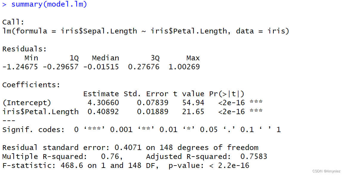
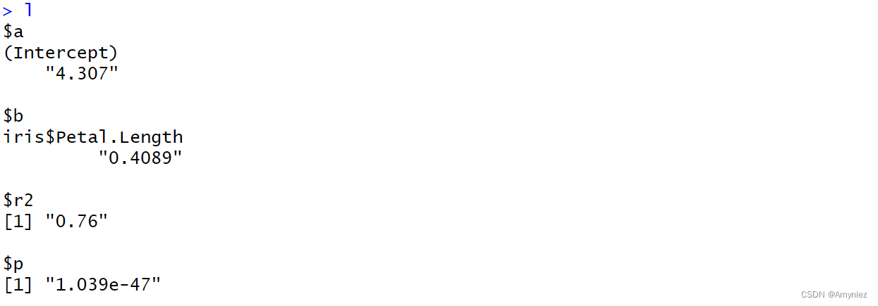
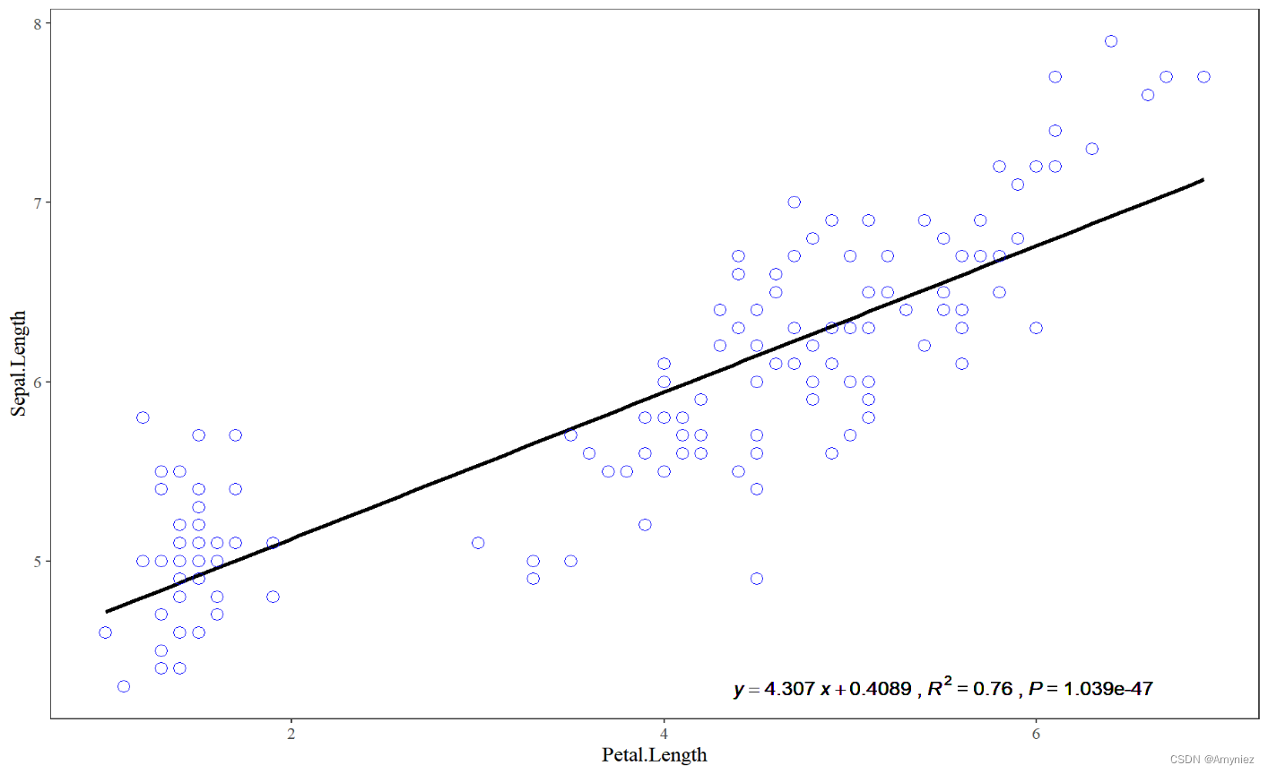
 文章介绍了如何使用R语言的lm函数对iris数据集进行线性拟合,并利用ggplot2库生成美观的拟合图像。通过代码示例展示了从模型构建到图像绘制,以及显著性分析的过程。


 1757
1757

 被折叠的 条评论
为什么被折叠?
被折叠的 条评论
为什么被折叠?
 到【灌水乐园】发言


