


{作为CNN学习入门的一部分,笔者在这里逐步给出UFLDL的各章节Exercise的个人代码实现,供大家参考指正}
理论部分可以在线参阅(页面最下方有中文选项)Linear Decoders 以及之前的 Autoencoders and Sparsity 部分内容
Note:
此章节的习题非常简单,区别于稀疏自编码,只需要对输出层的Error Term以及正向传播函数进行改写即可,输出层激励函数变为f(x)=x。
linearDecoderExercise.m
%% CS294A/CS294W Linear Decoder Exercise
% Instructions
% ------------
%
% This file contains code that helps you get started on the
% linear decoder exericse. For this exercise, you will only need to modify
% the code in sparseAutoencoderLinearCost.m. You will not need to modify
% any code in this file.
%%======================================================================
%% STEP 0: Initialization
% Here we initialize some parameters used for the exercise.
imageChannels = 3; % number of channels (rgb, so 3)
patchDim = 8; % patch dimension
numPatches = 100000; % number of patches
visibleSize = patchDim * patchDim * imageChannels; % number of input units
outputSize = visibleSize; % number of output units
hiddenSize = 400; % number of hidden units
sparsityParam = 0.035; % desired average activation of the hidden units.
lambda = 3e-3; % weight decay parameter
beta = 5; % weight of sparsity penalty term
epsilon = 0.1; % epsilon for ZCA whitening
%%======================================================================
%% STEP 1: Create and modify sparseAutoencoderLinearCost.m to use a linear decoder,
% and check gradients
% You should copy sparseAutoencoderCost.m from your earlier exercise
% and rename it to sparseAutoencoderLinearCost.m.
% Then you need to rename the function from sparseAutoencoderCost to
% sparseAutoencoderLinearCost, and modify it so that the sparse autoencoder
% uses a linear decoder instead. Once that is done, you should check
% your gradients to verify that they are correct.
% NOTE: Modify sparseAutoencoderCost first!
% To speed up gradient checking, we will use a reduced network and some
% dummy patches
% debugHiddenSize = 5;
% debugvisibleSize = 8;
% patches = rand([8 10]);
% theta = initializeParameters(debugHiddenSize, debugvisibleSize);
% [cost, grad] = sparseAutoencoderLinearCost(theta, debugvisibleSize, debugHiddenSize, ...
% lambda, sparsityParam, beta, ...
% patches);
% Check gradients
% numGrad = computeNumericalGradient( @(x) sparseAutoencoderLinearCost(x, debugvisibleSize, debugHiddenSize, ...
% lambda, sparsityParam, beta, ...
% patches), theta);
% Use this to visually compare the gradients side by side
% disp([numGrad grad]);
% diff = norm(numGrad-grad)/norm(numGrad+grad);
% Should be small. In our implementation, these values are usually less than 1e-9.
% disp(diff);
% assert(diff < 1e-9, 'Difference too large. Check your gradient computation again');
% Reach Here : 8.4135e-11
% NOTE: Once your gradients check out, you should run step 0 again to
% reinitialize the parameters
%}
%%======================================================================
%% STEP 2: Learn features on small patches
% In this step, you will use your sparse autoencoder (which now uses a
% linear decoder) to learn features on small patches sampled from related
% images.
%% STEP 2a: Load patches
% In this step, we load 100k patches sampled from the STL10 dataset and
% visualize them. Note that these patches have been scaled to [0,1]
load stlSampledPatches.mat
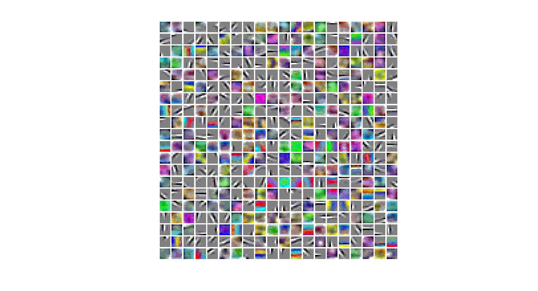
displayColorNetwork(patches(:, 1:100));
%% STEP 2b: Apply preprocessing
% In this sub-step, we preprocess the sampled patches, in particular,
% ZCA whitening them.
%
% In a later exercise on convolution and pooling, you will need to replicate
% exactly the preprocessing steps you apply to these patches before
% using the autoencoder to learn features on them. Hence, we will save the
% ZCA whitening and mean image matrices together with the learned features
% later on.
% Subtract mean patch (hence zeroing the mean of the patches)
meanPatch = mean(patches, 2);
patches = bsxfun(@minus, patches, meanPatch);
% Apply ZCA whitening
sigma = patches * patches' / numPatches;
[u, s, v] = svd(sigma);
ZCAWhite = u * diag(1 ./ sqrt(diag(s) + epsilon)) * u';
patches = ZCAWhite * patches;
displayColorNetwork(patches(:, 1:100));
%% STEP 2c: Learn features
% You will now use your sparse autoencoder (with linear decoder) to learn
% features on the preprocessed patches. This should take around 45 minutes.
theta = initializeParameters(hiddenSize, visibleSize);
% Use minFunc to minimize the function
addpath minFunc/
options = struct;
options.Method = 'lbfgs';
options.maxIter = 400;
options.display = 'on';
[optTheta, cost] = minFunc( @(p) sparseAutoencoderLinearCost(p, ...
visibleSize, hiddenSize, ...
lambda, sparsityParam, ...
beta, patches), ...
theta, options);
% Save the learned features and the preprocessing matrices for use in
% the later exercise on convolution and pooling
fprintf('Saving learned features and preprocessing matrices...\n');
save('STL10Features.mat', 'optTheta', 'ZCAWhite', 'meanPatch');
fprintf('Saved\n');
%% STEP 2d: Visualize learned features
W = reshape(optTheta(1:visibleSize * hiddenSize), hiddenSize, visibleSize);
b = optTheta(2*hiddenSize*visibleSize+1:2*hiddenSize*visibleSize+hiddenSize);
displayColorNetwork( (W*ZCAWhite)');
function [cost,grad] = sparseAutoencoderLinearCost(theta, visibleSize, hiddenSize, ...
                                                            lambda, sparsityParam, beta, data)
% -------------------- YOUR CODE HERE --------------------
% Instructions:
%   Copy sparseAutoencoderCost in sparseAutoencoderCost.m from your
%   earlier exercise onto this file, renaming the function to
%   sparseAutoencoderLinearCost, and changing the autoencoder to use a
%   linear decoder.
% -------------------- YOUR CODE HERE --------------------

W1 = reshape(theta(1:hiddenSize*visibleSize), hiddenSize, visibleSize);
W2 = reshape(theta(hiddenSize*visibleSize+1:2*hiddenSize*visibleSize), visibleSize, hiddenSize);
b1 = theta(2*hiddenSize*visibleSize+1:2*hiddenSize*visibleSize+hiddenSize);
b2 = theta(2*hiddenSize*visibleSize+hiddenSize+1:end);

dataSize = size(data, 2);

% define loss function:
% (1/2) * || y - H_w_b(x) || ^2 + Regularization term + Sparsity Constraint
MatrixZ2 = W1 * data + repmat(b1,1,dataSize);
MatrixA2 = 1 ./ (1 + exp(-MatrixZ2));
MatrixZ3 = W2 * MatrixA2 + repmat(b2,1,dataSize);
% MatrixA3 = 1 ./ (1 + exp(-MatrixZ3));
MatrixA3 = MatrixZ3; % Linear Decoder
MatrixDiff = MatrixA3 - data;
J_w_b_Vec = sum(MatrixDiff.^2)./2;

% Regularization term
WeightDecay = lambda/2 * (sum(sum(W1.^2)) + sum(sum(W2.^2)));
% Sparsity Constraint term
pVec = sum(MatrixA2,2)/dataSize; % row sum
KL = beta * sum(sparsityParam*(log(sparsityParam) - log(pVec)) ...
        + (1-sparsityParam)*(log(1-sparsityParam)-log(1-pVec)));

cost = sum(J_w_b_Vec)/dataSize + WeightDecay + KL;

% MatrixDelte_nl = -(data - MatrixA3).*(MatrixA3.*(1 - MatrixA3));
MatrixDelte_nl = -(data - MatrixA3);

MatrixDelte_hidden = ((W2)'*MatrixDelte_nl + ...
                        beta*(-sparsityParam./repmat(pVec,1,dataSize) + ...
                        (1-sparsityParam)./(1-repmat(pVec,1,dataSize)))).* ...
                        (MatrixA2.*(1 - MatrixA2));

% Compute the desired partial derivatives per layer
% Output Layer : nl
MatrixWLgradient_nl = MatrixDelte_nl * (MatrixA2)';
MatrixbLgradient_nl = sum(MatrixDelte_nl,2);
% Hidden Layer : nl - 1
MatrixWLgradient_hidden = MatrixDelte_hidden * (data)';
MatrixbLgradient_hidden = sum(MatrixDelte_hidden,2);

W1grad = MatrixWLgradient_hidden / dataSize + lambda * W1;
W2grad = MatrixWLgradient_nl / dataSize + lambda * W2;
b1grad = MatrixbLgradient_hidden / dataSize;
b2grad = MatrixbLgradient_nl / dataSize;

grad = [W1grad(:) ; W2grad(:) ; b1grad(:) ; b2grad(:)];

end
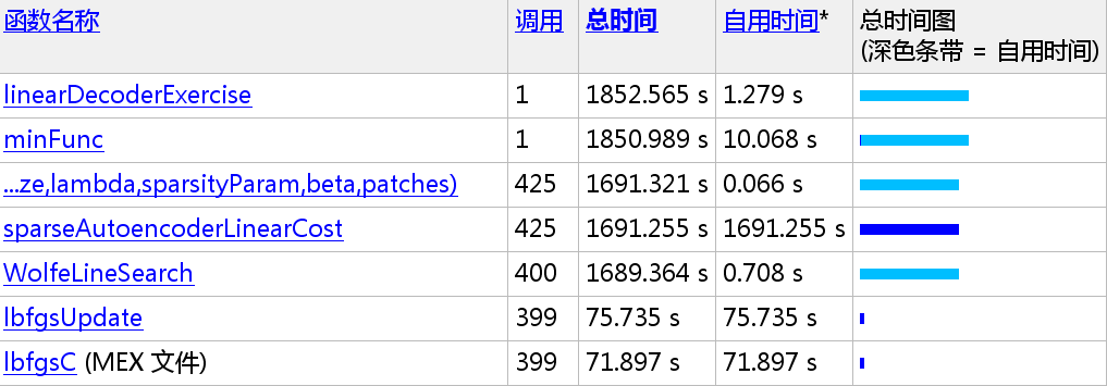
大约计算:1852.565 / 60 = 30.876 mins


 362
362

 被折叠的 条评论
为什么被折叠?
被折叠的 条评论
为什么被折叠?
 到【灌水乐园】发言


