Convolutional neural networks(CNN) (二) Sparse Autoencoder Exercise

{作为CNN学习入门的一部分，笔者在这里逐步给出UFLDL的各章节Exercise的个人代码实现，供大家参考指正}

理论部分可以在线参阅(页面最下方有中文选项)Neural Networks到Sparse AutoEncoder Notation部分内容，

也可以下载Andrew Ng的pdf。还是要先理解再去做exercise。

Exercise:Sparse Autoencoder实现如下：

train.m文件：

%% CS294A/CS294W Programming Assignment Starter Code

% As you may notice, the code which has been commented out with "Have already
% done." was part of the original code given by UFLDL. You may have to
% convert it executable code to complete your own exercise.

%  Instructions
%  ------------
% 
%  This file contains code that helps you get started on the
%  programming assignment. You will need to complete the code in sampleIMAGES.m,
%  sparseAutoencoderCost.m and computeNumericalGradient.m. 
%  For the purpose of completing the assignment, you do not need to
%  change the code in this file. 
%
%%======================================================================
%% STEP 0: Here we provide the relevant parameters values that will
%  allow your sparse autoencoder to get good filters; you do not need to 
%  change the parameters below.

visibleSize = 8*8;   % number of input units 

% WARNING !! Original value = 25. You may change it to test your gradient calculation result.
hiddenSize = 25;     % number of hidden units

sparsityParam = 0.01;   % desired average activation of the hidden units.
                     % (This was denoted by the Greek alphabet rho, which looks like a lower-case "p",
		     %  in the lecture notes). 
lambda = 0.0001;     % weight decay parameter       
beta = 3;            % weight of sparsity penalty term       

%%======================================================================
%% STEP 1: Implement sampleIMAGES
%
%  After implementing sampleIMAGES, the display_network command should
%  display a random sample of 200 patches from the dataset

patches = sampleIMAGES;

% display_network(patches(:,randi(size(patches,2),200,1)),8); 
% Have already done.


%  Obtain random parameters theta

% theta = initializeParameters(hiddenSize, visibleSize);
% Have already done.

%%======================================================================
%% STEP 2: Implement sparseAutoencoderCost
%
%  You can implement all of the components (squared error cost, weight decay term,
%  sparsity penalty) in the cost function at once, but it may be easier to do 
%  it step-by-step and run gradient checking (see STEP 3) after each step.  We 
%  suggest implementing the sparseAutoencoderCost function using the following steps:
%
%  (a) Implement forward propagation in your neural network, and implement the 
%      squared error term of the cost function.  Implement backpropagation to 
%      compute the derivatives.   Then (using lambda=beta=0), run Gradient Checking 
%      to verify that the calculations corresponding to the squared error cost 
%      term are correct.
%
%  (b) Add in the weight decay term (in both the cost function and the derivative
%      calculations), then re-run Gradient Checking to verify correctness. 
%
%  (c) Add in the sparsity penalty term, then re-run Gradient Checking to 
%      verify correctness.
%
%  Feel free to change the training settings when debugging your
%  code.  (For example, reducing the training set size or 
%  number of hidden units may make your code run faster; and setting beta 
%  and/or lambda to zero may be helpful for debugging.)  However, in your 
%  final submission of the visualized weights, please use parameters we 
%  gave in Step 0 above.

% [cost, grad] = sparseAutoencoderCost(theta, visibleSize, hiddenSize, lambda, ...
%                                     sparsityParam, beta, patches);
% Have already done.

%%======================================================================
%% STEP 3: Gradient Checking
%
% Hint: If you are debugging your code, performing gradient checking on smaller models 
% and smaller training sets (e.g., using only 10 training examples and 1-2 hidden 
% units) may speed things up.

% First, lets make sure your numerical gradient computation is correct for a
% simple function.  After you have implemented computeNumericalGradient.m,
% run the following: 

% checkNumericalGradient(); Have already done.

% Now we can use it to check your cost function and derivative calculations
% for the sparse autoencoder.  

% Have already done. {
% numgrad = computeNumericalGradient( @(x) sparseAutoencoderCost(x, visibleSize, ...
%                                                  hiddenSize, lambda, ...
%                                                  sparsityParam, beta, ...
%                                                  patches), theta);

% Use this to visually compare the gradients side by side
% disp([numgrad grad]); 

% Compare numerically computed gradients with the ones obtained from backpropagation
% diff = norm(numgrad-grad)/norm(numgrad+grad);
% disp(diff); % Should be small. In our implementation, these values are
            % usually less than 1e-9.

            % When you got this working, Congratulations!!! 
            
            % I got here @ 6.0098e-11 with Regularization term and sparsity
            % constraint.
% }
%%======================================================================
%% STEP 4: After verifying that your implementation of
%  sparseAutoencoderCost is correct, You can start training your sparse
%  autoencoder with minFunc (L-BFGS).

%  Randomly initialize the parameters
theta = initializeParameters(hiddenSize, visibleSize);

%  Use minFunc to minimize the function
addpath minFunc/
options.Method = 'lbfgs'; % Here, we use L-BFGS to optimize our cost
                          % function. Generally, for minFunc to work, you
                          % need a function pointer with two outputs: the
                          % function value and the gradient. In our problem,
                          % sparseAutoencoderCost.m satisfies this.
options.maxIter = 400;	  % Maximum number of iterations of L-BFGS to run 
options.display = 'on';


[opttheta, cost] = minFunc( @(p) sparseAutoencoderCost(p, ...
                                   visibleSize, hiddenSize, ...
                                   lambda, sparsityParam, ...
                                   beta, patches), ...
                              theta, options);

%%======================================================================
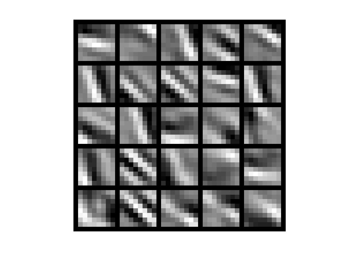
%% STEP 5: Visualization 

W1 = reshape(opttheta(1:hiddenSize*visibleSize), hiddenSize, visibleSize);
display_network(W1', 12); 

print -djpeg weights.jpg   % save the visualization to a file 

SparseAutoEncoderCost.m

function [cost,grad] = sparseAutoencoderCost(theta, visibleSize, hiddenSize, ...
                                             lambda, sparsityParam, beta, data)

% visibleSize: the number of input units (probably 64) 
% hiddenSize: the number of hidden units (probably 25) 
% lambda: weight decay parameter
% sparsityParam: The desired average activation for the hidden units (denoted in the lecture
%                           notes by the greek alphabet rho, which looks like a lower-case "p").
% beta: weight of sparsity penalty term
% data: Our 64x10000 matrix containing the training data.  So, data(:,i) is the i-th training example. 
  
% The input theta is a vector (because minFunc expects the parameters to be a vector). 
% We first convert theta to the (W1, W2, b1, b2) matrix/vector format, so that this 
% follows the notation convention of the lecture notes. 

W1 = reshape(theta(1:hiddenSize*visibleSize), hiddenSize, visibleSize);
W2 = reshape(theta(hiddenSize*visibleSize+1:2*hiddenSize*visibleSize), visibleSize, hiddenSize);
b1 = theta(2*hiddenSize*visibleSize+1:2*hiddenSize*visibleSize+hiddenSize);
b2 = theta(2*hiddenSize*visibleSize+hiddenSize+1:end);

% Cost and gradient variables (your code needs to compute these values). 
% Here, we initialize them to zeros. 
% cost = 0; No need to initialize cost.
% W1grad = zeros(size(W1)); 
% W2grad = zeros(size(W2));
% b1grad = zeros(size(b1)); 
% b2grad = zeros(size(b2));

%% ---------- YOUR CODE HERE --------------------------------------
%  Instructions: Compute the cost/optimization objective J_sparse(W,b) for the Sparse Autoencoder,
%                and the corresponding gradients W1grad, W2grad, b1grad, b2grad.
%
% W1grad, W2grad, b1grad and b2grad should be computed using backpropagation.
% Note that W1grad has the same dimensions as W1, b1grad has the same dimensions
% as b1, etc.  Your code should set W1grad to be the partial derivative of J_sparse(W,b) with
% respect to W1.  I.e., W1grad(i,j) should be the partial derivative of J_sparse(W,b) 
% with respect to the input parameter W1(i,j).  Thus, W1grad should be equal to the term 
% [(1/m) \Delta W^{(1)} + \lambda W^{(1)}] in the last block of pseudo-code in Section 2.2 
% of the lecture notes (and similarly for W2grad, b1grad, b2grad).
% 
% Stated differently, if we were using batch gradient descent to optimize the parameters,
% the gradient descent update to W1 would be W1 := W1 - alpha * W1grad, and similarly for W2, b1, b2. 
% 

dataSize = 10000;
% WARNING !! Original value = 10000. You may change it to test your gradient calculation result.
% dataSize = 10;

J_w_b_Vec = zeros(dataSize,1);
ActivationMatrix2 = zeros(hiddenSize, dataSize); % activation equals output
ActivationMatrix3 = zeros(visibleSize, dataSize); % activation equals output

DelteW1 = zeros(size(W1)); 
DelteW2 = zeros(size(W2)); 
Delteb1 = zeros(size(b1)); 
Delteb2 = zeros(size(b2)); 

% define loss function: (1/2) * || y - H_w_b(x) || ^2
for i = 1:1:dataSize
    z2 = W1 * data(:,i) + b1;
    a2 = sigmoid(z2);
    ActivationMatrix2(:,i) = a2;
    z3 = W2 * a2 + b2;
    a3 = sigmoid(z3);
    ActivationMatrix3(:,i) = a3;
    diff = a3 - data(:,i);
    J_w_b_Vec(i) = sum((diff.^2))/2;
end

% Regularization term
WeightDecay = lambda/2 * (sum(sum(W1.^2)) + sum(sum(W2.^2)));
% Sparsity Constraint term
pVec = sum(ActivationMatrix2,2)/dataSize; % row sum
KL = beta * sparsityConstraint(sparsityParam, pVec);

cost = sum(J_w_b_Vec)/dataSize + WeightDecay + KL;

for i = 1:1:dataSize
    [dW1, db1, dW2, db2] = singleSampleGradient(data(:,i), ...
                                                ActivationMatrix2(:,i), ...
                                                ActivationMatrix3(:,i), ...
                                                W2, ...
                                                beta, ...
                                                pVec, ...
                                                sparsityParam);
    DelteW1 = DelteW1 + dW1;
    DelteW2 = DelteW2 + dW2;
    Delteb1 = Delteb1 + db1;
    Delteb2 = Delteb2 + db2;
    
end

W1grad = DelteW1 / dataSize + lambda * W1;
W2grad = DelteW2 / dataSize + lambda * W2;
b1grad = Delteb1 / dataSize;
b2grad = Delteb2 / dataSize;

%-------------------------------------------------------------------
% After computing the cost and gradient, we will convert the gradients back
% to a vector format (suitable for minFunc).  Specifically, we will unroll
% your gradient matrices into a vector.

grad = [W1grad(:) ; W2grad(:) ; b1grad(:) ; b2grad(:)];

end

%-------------------------------------------------------------------
% Here's an implementation of the sigmoid function, which you may find useful
% in your computation of the costs and the gradients.  This inputs a (row or
% column) vector (say (z1, z2, z3)) and returns (f(z1), f(z2), f(z3)). 

function sigm = sigmoid(x)
  
sigm = 1 ./ (1 + exp(-x));
end

% Single Sample
function [WLgradient_hidden, bLgradient_hidden, WLgradient_nl, bLgradient_nl] = ...
    singleSampleGradient(data, ActivationVec_hidden, ActivationVec_nl, W2, beta, pVec, sparsityParam)

% Delte_nl = zeros(size(ActivationVec_nl)); 
% Delte_hidden = zeros(size(ActivationVec_hidden));

% Compute error terms per layer
% Output Layer : nl
Delte_nl = -(data - ActivationVec_nl).*(ActivationVec_nl.*(1 - ActivationVec_nl));
% Hidden Layer : nl - 1 without sparsity constraint
% Delte_hidden = ((W2)'*Delte_nl).*(ActivationVec_hidden.*(1 - ActivationVec_hidden));
% Hidden Layer : nl - 1 with sparsity constraint
Delte_hidden = ((W2)'*Delte_nl + beta*(-sparsityParam./pVec + (1-sparsityParam)./(1-pVec))).* ...
    (ActivationVec_hidden.*(1 - ActivationVec_hidden));

% Compute the desired partial derivatives per layer
% Output Layer : nl
WLgradient_nl = Delte_nl * (ActivationVec_hidden)';
bLgradient_nl = Delte_nl;
% Hidden Layer : nl - 1
WLgradient_hidden = Delte_hidden * (data)';
bLgradient_hidden = Delte_hidden;

end

% Sparsity Constraint
function KL = sparsityConstraint(sparsityParam, pVec)

KL = sum(sparsityParam*(log(sparsityParam) - log(pVec)) ...
        + (1-sparsityParam)*(log(1-sparsityParam)-log(1-pVec)));  

end

smapleIMAGES.m

function patches = sampleIMAGES()
% sampleIMAGES
% Returns 10000 patches for training

load IMAGES;    % load images from disk 

patchsize = 8;  % we'll use 8x8 patches 
numpatches = 10000;

% Initialize patches with zeros.  Your code will fill in this matrix--one
% column per patch, 10000 columns. 
patches = zeros(patchsize*patchsize, numpatches);

%% ---------- YOUR CODE HERE --------------------------------------
%  Instructions: Fill in the variable called "patches" using data 
%  from IMAGES.  
%  
%  IMAGES is a 3D array containing 10 images
%  For instance, IMAGES(:,:,6) is a 512x512 array containing the 6th image,
%  and you can type "imagesc(IMAGES(:,:,6)), colormap gray;" to visualize
%  it. (The contrast on these images look a bit off because they have
%  been preprocessed using using "whitening."  See the lecture notes for
%  more details.) As a second example, IMAGES(21:30,21:30,1) is an image
%  patch corresponding to the pixels in the block (21,21) to (30,30) of
%  Image 1

% patch64 = zeros(patchsize, patchsize); 
% As you may notice, preallocation was not recommended here.
randompick = 3; % Just pick the third Pic in the DataSet.
for i = 1:1:100
    for j = 1:1:100
        patch64 = IMAGES(i:i+7,j:j+7,randompick);
        patches(:,100*(i-1)+j) = patch64(:);
    end
end

%% ---------------------------------------------------------------
% For the autoencoder to work well we need to normalize the data
% Specifically, since the output of the network is bounded between [0,1]
% (due to the sigmoid activation function), we have to make sure 
% the range of pixel values is also bounded between [0,1]
patches = normalizeData(patches);

end


%% ---------------------------------------------------------------
function patches = normalizeData(patches)

% Squash data to [0.1, 0.9] since we use sigmoid as the activation
% function in the output layer

% Remove DC (mean of images). 
patches = bsxfun(@minus, patches, mean(patches));

% Truncate to +/-3 standard deviations and scale to -1 to 1
pstd = 3 * std(patches(:));
patches = max(min(patches, pstd), -pstd) / pstd;

% Rescale from [-1,1] to [0.1,0.9]
patches = (patches + 1) * 0.4 + 0.1;

end

ComputeNumericalGradient.m

function numgrad = computeNumericalGradient(J, theta)
% numgrad = computeNumericalGradient(J, theta)
% theta: a vector of parameters
% J: a function that outputs a real-number. Calling y = J(theta) will return the
% function value at theta. 
  
% Initialize numgrad with zeros
% numgrad = zeros(size(theta));

%% ---------- YOUR CODE HERE --------------------------------------
% Instructions: 
% Implement numerical gradient checking, and return the result in numgrad.  
% (See Section 2.3 of the lecture notes.)
% You should write code so that numgrad(i) is (the numerical approximation to) the 
% partial derivative of J with respect to the i-th input argument, evaluated at theta.  
% I.e., numgrad(i) should be the (approximately) the partial derivative of J with 
% respect to theta(i).
%                
% Hint: You will probably want to compute the elements of numgrad one at a time. 
EPSILON = 1e-4;
numgrad = (Jelement2vecFunction(J, theta, EPSILON) - Jelement2vecFunction(J, theta, -EPSILON))/(2*EPSILON);

%% ---------------------------------------------------------------
end

%% 
% Instruction:
% Input: vector
% Output: vector
% J: Function mentioned above
function vec = Jelement2vecFunction(J, theta, bias)
    vec = zeros(size(theta));
    for i = 1:size(theta,1)
        theta(i) = theta(i) + bias;
        vec(i) = J(theta);
        theta(i) = theta(i) - bias;
    end
end

Result: 每个人得出的结果 可能会有所不同，更多细节还请查看 这里。