从细节过渡到实例 一天学会Pytorch

1. PyTorch基础

1.1. 导入PyTorch包

import torch

1.2. 张量的初始化

(1) 创建并初始化张量

# 创建一个任意张量
tensor = torch.tensor([5.5, 3, 0])
'''
tensor([5.5000, 3.0000, 0.0000])
'''

# 创建一个数列张量，从1开始，到10结束，间隔为2
tensor_arange = torch.arange(1, 10, 2)
'''
tensor([1, 3, 5, 7, 9])
'''

# 创建一个空张量，大小为 5*3
tensor_empty = torch.empty((5, 3))
'''
tensor([[7.1819e+22, 4.0666e+21, 1.0999e+27],
        [2.6277e+17, 7.2368e+25, 2.7516e+17],
        [4.4721e+21, 1.8497e+31, 2.6845e+17],
        [4.4724e+21, 1.8497e+31, 5.4214e-11],
        [9.1720e-04, 1.9086e-41, 0.0000e+00]])
'''

# 创建一个0张量，大小为 5*3
tensor_zeros = torch.zeros((5, 3))
'''
tensor([[0., 0., 0.],
        [0., 0., 0.],
        [0., 0., 0.],
        [0., 0., 0.],
        [0., 0., 0.]])
'''

# 创建一个1张量，大小为 5*3
tensor_ones = torch.ones((5, 3))
'''
tensor([[1., 1., 1.],
        [1., 1., 1.],
        [1., 1., 1.],
        [1., 1., 1.],
        [1., 1., 1.]])
'''

# 创建一个任意值张量，大小为 5*3，填充值为99
tensor_full = torch.full([5, 3], 99.) 
'''
tensor([[99., 99., 99.],
        [99., 99., 99.],
        [99., 99., 99.],
        [99., 99., 99.],
        [99., 99., 99.]])
'''

# 创建一个在[0,1)内均匀分布的随机张量，大小为 5*3
tensor_rand = torch.rand((5, 3))
'''
tensor([[0.4991, 0.5687, 0.9626],
        [0.3185, 0.2407, 0.6076],
        [0.2600, 0.0289, 0.1632],
        [0.4269, 0.9201, 0.4774],
        [0.7576, 0.9349, 0.5644]])
'''

# 创建一个服从标准正态分布的随机张量，大小为 5*3
tensor_randn = torch.randn((5, 3))
'''
tensor([[-0.6753, -1.6975, -1.1010],
        [-1.9736,  0.6005,  0.5844],
        [ 0.3015, -0.5700,  1.1196],
        [ 0.3156, -0.4194, -0.8618],
        [-1.1506,  0.5248,  0.0401]])
'''

# 创建一个服从均值为mean、标准差为std正态分布的随机张量，大小为 1*10
# 更多关于随机正态分布张量的内容：https://pytorch.org/docs/stable/generated/torch.normal.html#torch-normal
tensor_normal = torch.normal(mean=torch.arange(0., 1.), std=torch.arange(0, 10, 1))
'''
tensor([  0.0000,  -0.9662,  -0.2848,   5.5105,   0.9495,   3.0639,  -3.4798,
          6.9719, -11.6149,  -6.0056])
'''

(2) 从已有张量创建大小一致的张量

# 根据已有的张量创建大小一致的0张量
tensor_zeros = torch.zeros_like(tensor_empty)
'''
tensor([[0., 0., 0.],
        [0., 0., 0.],
        [0., 0., 0.],
        [0., 0., 0.],
        [0., 0., 0.]])
'''

# 根据已有的张量创建大小一致的1张量
tensor_ones = torch.ones_like(tensor_empty)
'''
tensor([[1., 1., 1.],
        [1., 1., 1.],
        [1., 1., 1.],
        [1., 1., 1.],
        [1., 1., 1.]])
'''

# 根据已有的张量创建大小一致在[0,1)内的均匀分布的随机张量
tensor_rand = torch.rand_like(tensor_empty)
'''
tensor([[0.0437, 0.9776, 0.1685],
        [0.5190, 0.6811, 0.3768],
        [0.4864, 0.7169, 0.4813],
        [0.4596, 0.4703, 0.2497],
        [0.9778, 0.9880, 0.9152]])
'''

(3) 指定张量的数据类型 dtype

# 创建long数据类型的张量
tensor_long = torch.ones((5, 3), dtype=torch.long)
'''
tensor([[1, 1, 1, 1, 1]])
'''

# 查看张量的数据类型
print(tensor_long.dtype)
'''
torch.int64
'''

# 改变张量的数据类型
print(tensor_long.float())
'''
torch.float32
'''

# 张量的数据类型总结：
# 8位无符号整型：torch.uint8
# 8位整型：torch.int8
# 16位整型：torch.int16 | torch.short
# 32位整型：torch.int32 | torch.int
# 64位整型：torch.int64 | torch.long
# 16位浮点型：torch.float16 | torch.half
# 32位浮点型：torch.float32 | torch.float
# 64位浮点型：torch.float64 | torch.double

1.3. 张量的基本操作

(1) 查看张量的大小

tensor_empty = torch.empty((5, 3))
print(tensor_empty.size())
'''
torch.Size([5, 3])
'''

print(tensor_empty.shape)
'''
torch.Size([5, 3])
'''

(2) 张量堆叠

# 创建一个空张量，大小为 5*3
tensor_empty = torch.tensor([[1,2,3]])
'''
tensor([[1, 2, 3]])
'''

# 张量按维度0堆叠，即添加行
tensor_cat0 = torch.cat((tensor_empty,tensor_empty,tensor_empty), 0)
'''
tensor([[1, 2, 3],
        [1, 2, 3],
        [1, 2, 3]])
'''

# 张量按维度0堆叠，即添加列
tensor_cat1 = torch.cat((tensor_empty,tensor_empty,tensor_empty), 1)
'''
tensor([[1, 2, 3, 1, 2, 3, 1, 2, 3]])
'''

(3) 张量增减维度

tensor_zeros = torch.zeros(3, 2, 4, 1, 2, 1)
print(tensor_zeros.shape)
'''
torch.Size([3, 2, 4, 1, 2, 1])
'''

# 在张量的第dim维增添一个维数为1的维度
tensor_unsqueeze = torch.unsqueeze(tensor_zeros, dim=0)
print(tensor_unsqueeze.shape)
'''
torch.Size([1, 3, 2, 4, 1, 2, 1])
'''

# 删去张量中维数为1的维度，如果未指定dim则删去全部维数为1的维度
tensor_squeeze = torch.squeeze(tensor_zeros, dim=3)
print(tensor_squeeze.shape)
'''
torch.Size([3, 2, 4, 2, 1])
'''

(4) 张量分割

# 创建一个数列张量
tensor_arange = torch.arange(10)
'''
tensor([0, 1, 2, 3, 4, 5, 6, 7, 8, 9])
'''

# 把张量均匀分割。4表示分割成4份；dim=0表示按行分割，dim=1表示按列分割
tensor_chunk = torch.chunk(tensor_arange, 4, dim=0)
'''
(tensor([0, 1, 2]), tensor([3, 4, 5]), tensor([6, 7, 8]), tensor([9]))
'''

# 把张量按指定方案分割。[1,2,3,4]表示分割成4份，每份分别有1、2、3、4个元素；dim=0表示按行分割，dim=1表示按列分割
tensor_split = torch.split(tensor_arange, [1,2,3,4], dim=0)
'''
(tensor([0]), tensor([1, 2]), tensor([3, 4, 5]), tensor([6, 7, 8, 9]))
'''

(5) 选择张量中的元素

# 创建一个随机张量
tensor_randn = torch.randn((5, 3))
'''
tensor([[ 0.3567,  1.3366,  0.1045],
        [ 0.7795, -0.2843, -0.2252],
        [-0.4905, -0.2118, -1.5967],
        [ 0.8375,  0.3417, -0.7932],
        [-0.5923, -2.4375, -0.9357]])
'''

# 取张量的(0,0)元素
print(tensor_randn[0, 0])
'''
tensor(0.3567)
'''

# 取张量的第一列元素
print(tensor_randn[:, 0])
'''
tensor([ 0.3567,  0.7795, -0.4905,  0.8375, -0.5923])
'''

# 选择张量中行index为0、2、4的元素
print(torch.index_select(tensor_randn, dim=0, index=torch.tensor([0, 2, 4])))
'''
tensor([[ 0.3567,  1.3366,  0.1045],
        [-0.4905, -0.2118, -1.5967],
        [-0.5923, -2.4375, -0.9357]])
'''

# 选择张量中>=0的元素，mask为条件表达式
print(torch.masked_select(tensor_randn, mask=tensor_randn.ge(0)))
'''
tensor([0.3567, 1.3366, 0.1045, 0.7795, 0.8375, 0.3417])
'''

(6) 改变张量形状

# 创建一个随机张量
tensor_randn = torch.randn((5, 3))
'''
tensor([[ 0.3478, -2.1573,  0.7693],
        [-0.3915, -1.2390, -0.7590],
        [-0.3685,  0.1261,  0.1424],
        [ 0.5710,  0.0483, -1.2647],
        [-0.8762,  0.9870, -0.0174]])
'''

# 将tensor_randn从(5,3)转变为(3,5)
tensor_reshape = torch.reshape(tensor_randn, (3,5))
'''
tensor([[ 0.3478, -2.1573,  0.7693, -0.3915, -1.2390],
        [-0.7590, -0.3685,  0.1261,  0.1424,  0.5710],
        [ 0.0483, -1.2647, -0.8762,  0.9870, -0.0174]])
'''

# 将tensor_randn从(5,3)转变为(3,5)
tensor_view = tensor_randn.view((-1,5)) #当某一维是-1时，会根据另一维自动计算它的大小
'''
tensor([[ 0.3478, -2.1573,  0.7693, -0.3915, -1.2390],
        [-0.7590, -0.3685,  0.1261,  0.1424,  0.5710],
        [ 0.0483, -1.2647, -0.8762,  0.9870, -0.0174]])
'''

(7) 张量运算

# 创建一个数列张量
tensor_arange1 = torch.arange(10, 20, 2)
tensor_arange2 = torch.arange(0, -10, -2)
'''
tensor([10., 12., 14., 16., 18.])
tensor([-1., -3., -5., -7., -9.])
'''

# 张量元素相加 + 两种方法
tensor_add = torch.add(tensor_arange1,tensor_arange2, out=None)
# torch.add(tensor_arange1,tensor_arange2, out=tensor_arange1) # 此时操作结果直接存储在tensor_arange1中
# tensor_arange2.add_(tensor_arange1) # 此时操作结果直接存储在tensor_arange2中
'''
tensor([9., 9., 9., 9., 9.])
'''

# 张量元素相乘 ×
tensor_mul = torch.mul(tensor_arange1, tensor_arange2, out=None)
'''
tensor([ -10.,  -36.,  -70., -112., -162.])
'''

# 张量元素相除 ÷ 这里要注意除法的结果一般为浮点数，所以张量类型也应当为浮点数类型
tensor_div = torch.div(tensor_arange1, tensor_arange2, out=None)
'''
tensor([-10.0000,  -4.0000,  -2.8000,  -2.2857,  -2.0000])
'''

# 张量元素求幂 ^
tensor_pow = torch.pow(tensor_arange1, tensor_arange2, out=None)
'''
tensor([1.0000e-01, 5.7870e-04, 1.8593e-06, 3.7253e-09, 5.0414e-12])
'''

# 张量元素开平方根 √
tensor_sqrt = torch.sqrt(tensor_arange1, out=None)
'''
tensor([3.1623, 3.4641, 3.7417, 4.0000, 4.2426])
'''

# 张量元素四舍五入
tensor_round = torch.round(tensor_arange1, out=None)
'''
tensor([10., 12., 14., 16., 18.])
'''

# 张量元素取绝对值
tensor_abs = torch.abs(tensor_arange2, out=None)
'''
tensor([1., 3., 5., 7., 9.])
'''

# 张量元素向上取整，等于向下取整+1
tensor_ceil = torch.ceil(tensor_arange2, out=None)
'''
tensor([-1., -3., -5., -7., -9.])
'''

# 张量元素限定值域，把输入数据规范在min-max区间，超过范围的用min、max代替
tensor_clamp = torch.clamp(tensor_arange1, min=12, max=16, out=None)
'''
tensor([12., 12., 14., 16., 16.])
'''

# 张量取最大值的下标，dim=1时取出每一列中的最大值的下标，dim=0时取出每一行中的最大值的下标
tensor_argmax = torch.argmax(tensor_arange1, dim=0, keepdim=False)
'''
tensor(4)
'''

# 张量元素输入sigmoid函数进行处理
tensor_sigmoid = torch.sigmoid(tensor_arange1, out=None)
'''
tensor([1.0000, 1.0000, 1.0000, 1.0000, 1.0000])
'''

# 张量元素输入tanh函数进行处理
tensor_tanh = torch.tanh(tensor_arange1, out=None)
'''
tensor([1., 1., 1., 1., 1.])
'''

1.4. Tensor与Numpy、List的互相转换

(1) Tensor 转 Numpy 再转 List

# 创建一个1张量
tensor_ones = torch.ones((2,4))
'''
tensor([[1., 1., 1., 1.],
        [1., 1., 1., 1.]])
'''

# 将tensor张量转换为array数组
# 转换后，numpy的变量和原来的tensor会共用底层内存地址，所以如果原来的tensor改变了，numpy变量也会随之改变
tensor_numpy = tensor_ones.numpy()
'''
[[1. 1. 1. 1.]
 [1. 1. 1. 1.]]
'''

tensor_list = tensor_numpy.tolist()
'''
[[1., 1., 1., 1.],
 [1., 1., 1., 1.]]
'''

(2) List 转 Numpy 再转 Tensor

# 创建一个1列表
list_ones = [1 for i in range(0, 5)]
'''
[1, 1, 1, 1, 1]
'''

# 将list转换为array
array_ones = numpy.array(list_ones)
'''
[1 1 1 1 1]
'''

# 将array数组转换为tensor张量
# 转换后，tensor和原来的numpy的变量会共用底层内存地址，所以如果原来的tensor改变了，numpy变量也会随之改变
tensor_form_numpy = torch.from_numpy(array_ones)
'''
tensor([1., 1., 1., 1., 1.], dtype=torch.int)
'''

# 改变tensor的数据类型
tensor_form_numpy = tensor_form_numpy.float()
'''
tensor([1., 1., 1., 1., 1.], dtype=torch.float32)
'''

1.5. GPU加速

在Pytorch使用GPU进行加速之前，需要先安装机器显卡对应的 CUDA ，然后即可利用GPU进行运算

(1) 将数据从CPU迁入GPU

# 一般而言，我们将网络模型、损失函数、张量三种数据迁入GPU中进行加速
# 将网络模型和损失函数迁入GPU
net = Net()
loss_func = torch.nn.CrossEntropyLoss()

if(torch.cuda.is_available()):
    net = net.cuda()
    loss_func = loss_func.cuda()

# 将张量迁入GPU，实际上只需要将输入网络的张量数据迁入GPU即可，因为根据这些数据产生的中间数据以及预测结果均在GPU中，所以只要把握住源头数据，后面的数据就不需要再显式地迁入GPU
# 有些旧版的Pytorch需要将张量封装成Variable类型才可以迁入GPU，不过这已经是过去式了
if (torch.cuda.is_available()):
    tensor_x, tensor_y = tensor_x.cuda(), tensor_y.cuda()
    # tensor_x, tensor_y = Variable(tensor_x).cuda(), Variable(tensor_y).cuda() # 旧版Pytorch

(2) 将数据从GPU迁出到CPU

# 将网络模型预测的结果迁出GPU，一般是最终损失值、精确度，也可以是其他迁入了GPU的数据
if(torch.cuda.is_available()):
    loss = loss.cpu()
    accurate = accurate.cpu()

2. 自动微分

2.1. 开启自动微分

# 创建一个张量并在初始化时设置requires_grad=True开启自动微分功能
tensor_ones = torch.ones(2, 2, requires_grad=True)
'''
tensor([[1., 1.],
        [1., 1.]], requires_grad=True)
'''

# 创建一个张量，初始化时不开启自动微分
tensor_randn = torch.randn(2, 2)
tensor_randn = (tensor_randn * 3) / (tensor_randn - 1)
print(tensor_randn.requires_grad)

# 设置该张量为自动微分
tensor_randn.requires_grad_(True)
print(tensor_randn.requires_grad)
'''
False
True
'''

2.2. 梯度计算

(1) 查看梯度方程 grad_fn

# 创建一个1张量，并查看其梯度方程grad_fn
tensor_ones = torch.ones(2, 2, requires_grad=True)
print(tensor_ones)
print(tensor_ones.grad_fn) # 可以看到，单独的张量是没有梯度方程的
'''
tensor([[1., 1.],
        [1., 1.]], requires_grad=True)
None
'''

# 构建一个张量方程，并查看其梯度方程grad_fn
tensor_add = tensor_ones + 2
print(tensor_add)
print(tensor_add.grad_fn) # 该张量方程是由加法构建的张量方程，因此梯度方程是AddBackward类型的
'''
tensor([[3., 3.],
        [3., 3.]], grad_fn=<AddBackward0>)
<AddBackward0 object at 0x00000245B1025CA0>
'''

# 构建一个张量方程，并查看其梯度方程grad_fn
tensor_mul = tensor_ones * tensor_ones * 2
print(tensor_mul)
print(tensor_mul.grad_fn) # 该张量方程是由乘法构建的张量方程，因此梯度方程是MulBackward类型的
'''
tensor([[2., 2.],
        [2., 2.]], grad_fn=<MulBackward0>)
<MulBackward0 object at 0x000001A309525CA0>
'''

(2) 反向传播计算标量梯度

# 创建一个1张量
tensor_x = torch.ones(2, 2, requires_grad=True)
tensor_y = tensor_x + 2
tensor_z = tensor_y * tensor_y * 3
out = tensor_z.mean()
print(out)
'''
tensor(27., grad_fn=<MeanBackward0>)
'''

# 反向传播计算梯度
# out是标量，因此不需要为backward()函数指定参数,相当于out.backward(torch.tensor(1))
out.backward() 
print(tensor_x.grad) # 输出梯度
'''
tensor([[4.5000, 4.5000],
        [4.5000, 4.5000]])
'''

(3) 反向传播计算矢量梯度

# 创建一个随机张量
tensor_x = torch.randn((1,3), requires_grad=True)
print(tensor_x)
'''
tensor([[0.2427, 0.8484, 0.7631]], requires_grad=True)
'''

# 求 y^(2^(n))>=1000 的最小值
tensor_y = tensor_x * 2
while tensor_y.data.norm() < 1000: 
    tensor_y = tensor_y * 2
print(tensor_y)
'''
tensor([[248.5333, 868.7134, 781.4405]], grad_fn=<MulBackward0>)
'''

gradients = torch.tensor([[0.1, 1.0, 0.0001]], dtype=torch.float) # 梯度参数
tensor_y.backward(gradients) # 对矢量进行梯度计算需要指定梯度，tensor_x[0,0]与tensor_y[0,0]对应梯度0.1...
print(tensor_x.grad)
'''
tensor([[102.40, 1024.0, 0.10240]])
'''

(4) 不进行梯度计算

# 创建一个随机张量
tensor_x = torch.randn((1,3), requires_grad=True)
print(tensor_x.requires_grad)
'''
True
'''

# 进行梯度计算
tensor_y = tensor_x ** 2
print(tensor_y.requires_grad)
'''
True
'''

# 将变量包裹在no_grad()中，可以不进行梯度计算
with torch.no_grad():
    tensor_y = tensor_x ** 2
    print(tensor_y.requires_grad)
'''
False
'''

(5) 切断梯度计算

# 创建一个随机张量
tensor_x = torch.randn(3, requires_grad=True)
tensor_y = tensor_x ** 2
print(tensor_x.requires_grad)
print(tensor_y.requires_grad)
'''
True
True
'''

# 切断tensor_y的梯度计算
tensor_y = tensor_y.detach()
print(tensor_y.requires_grad)
'''
False
'''

3. 神经网络要素

3.1. 构建网络

(1) 使用torch.nn模块构建神经网络

关于torch.nn模块包含的全部方法在官方文档 torch.nn 中有详细介绍。翻译版可以在 PyTorch中的torch.nn模块使用详解 中查看

import torch
import torch.nn as nn
import torch.nn.functional as F

class Net(nn.Module):
    #定义Net的初始化函数，这个函数定义了该神经网络的基本结构
    def __init__(self):
        super(Net, self).__init__() #复制并使用Net的父类的初始化方法，即先运行nn.Module的初始化函数
        self.conv1 = nn.Conv2d(3, 6, 5) # 定义二维卷积层：输入为3通道图像,输出6个特征图, 卷积核为5x5正方形
        self.conv2 = nn.Conv2d(6, 16, 5)# 定义二维卷积层：输入为6张特征图,输出16个特征图, 卷积核为5x5正方形
        self.fc1   = nn.Linear(16*5*5, 120) # 定义线性全连接层：y = Wx + b，并将16*5*5个特征连接到120个节点上
        self.fc2   = nn.Linear(120, 84)#定义线性全连接层：y = Wx + b，并将120个节点连接到84个节点上
        self.fc3   = nn.Linear(84, 10)#定义线性全连接层：y = Wx + b，并将84个节点连接到10个节点上

    #定义该神经网络的向前计算函数，该函数定义成功后，会自动生成反向传播函数（autograd）
    def forward(self, x):
        x = F.max_pool2d(F.relu(self.conv1(x)), (2, 2)) #输入x经过卷积conv1之后，经过激活函数ReLU（原来这个词是激活函数的意思），使用2x2的窗口进行最大池化Max pooling，然后更新到x。
        x = F.max_pool2d(F.relu(self.conv2(x)), 2) #输入x经过卷积conv2之后，经过激活函数ReLU，使用2x2的窗口进行最大池化Max pooling，然后更新到x。
        x = x.view(-1, 16*5*5) #view函数将张量x变形成一维的向量形式，总特征数并不改变，为接下来的全连接作准备，可验算这里的-1值为32。。
        x = F.relu(self.fc1(x)) #输入x经过全连接1，再经过ReLU激活函数处理，然后更新x
        x = F.relu(self.fc2(x)) #输入x经过全连接2，再经过ReLU激活函数处理，然后更新x
        x = self.fc3(x) #输入x经过全连接3处理，然后更新x
        return x

(2) 查看神经网络的参数

# 实例化一个神经网络
net = Net()
layers = list(net.parameters())

# 查看神经网络的基本结构信息
print(net)
'''
Net(
  (conv1): Conv2d(3, 6, kernel_size=(5, 5), stride=(1, 1))
  (conv2): Conv2d(6, 16, kernel_size=(5, 5), stride=(1, 1))
  (fc1): Linear(in_features=400, out_features=120, bias=True)
  (fc2): Linear(in_features=120, out_features=84, bias=True)
  (fc3): Linear(in_features=84, out_features=10, bias=True)
)
'''

# 查看神经网络的总层数
print(len(layers)) 
'''
10
'''

# 查看最后一层的参数
print(layers[-1]) 
'''
Parameter containing:
tensor([-0.0674,  0.0600,  0.0800, -0.0760,  0.0293,  0.0745,  0.0182,  0.0616,
        -0.0197,  0.0729], requires_grad=True)
'''

# 查看第一层的大小
print(layers[0].size()) 
'''
torch.Size([6, 3, 5, 5])
'''

# 查看每一层的参数和节点数量
total_parameter=0
layer_num = 1
for layer in layers:
    parameter = 1
    for _ in layer.size():
        parameter *= _
    print("第" + str(layer_num) + "层的结构："+ str(list(layer.size())) + "，参数和："+ str(parameter))
    total_parameter = total_parameter + parameter
    layer_num += 1
print("总参数和："+ str(total_parameter))
'''
第1层的结构：[6, 3, 5, 5]，参数和：450
第2层的结构：[6]，参数和：6
第3层的结构：[16, 6, 5, 5]，参数和：2400
第4层的结构：[16]，参数和：16
第5层的结构：[120, 400]，参数和：48000
第6层的结构：[120]，参数和：120
第7层的结构：[84, 120]，参数和：10080
第8层的结构：[84]，参数和：84
第9层的结构：[10, 84]，参数和：840
第10层的结构：[10]，参数和：10
总参数和：62006

Process finished with exit code 0

'''

(3) 查看前向计算过程

# 实例化一个神经网络
net = Net()
input = torch.randn(2, 3, 32, 32) # 产生2个3通道，32*32的随机输入，这是nn.Conv2d的接收格式
out = net(input)
print(out)
'''
tensor([[-0.1063,  0.0641, -0.0391, -0.0517,  0.1174, -0.0600,  0.0044, -0.0311,
         -0.1074,  0.0226],
        [-0.0779,  0.0697, -0.0486, -0.0842,  0.1377, -0.0276, -0.0247, -0.0504,
         -0.1054,  0.0065]], grad_fn=<AddmmBackward>)
'''

(4) 查看反向传播过程

net = Net() # 实例化一个神经网络
net.zero_grad() # 梯度初始化

input = torch.randn(1, 3, 32, 32) 
out = net(input)

out.backward(torch.randn(1, 10)) # 随机选取参数进行反向传播
print(out)

'''
tensor([[-0.0829,  0.0556, -0.0088, -0.0263, -0.0518,  0.0802, -0.0923,  0.0091,
          0.0122,  0.0927]], grad_fn=<AddmmBackward>)
'''

3.2. 损失函数

(1) 定义损失函数并计算损失

net = Net()
criterion = nn.MSELoss() # 定义均方误差损失函数
target = torch.randn(10).view(1, -1)  # 定义10个随机真值（因为网络最后一层有10个输出），并转换为行向量
print(target)
'''
tensor([[-1.1115, -0.3807,  0.5877, -1.0567, -0.0541, -0.3390, -1.9487, -0.2775,
         -0.0366,  0.7521]])
'''

output = net(torch.randn(1, 3, 32, 32))  # 用随机输入计算输出
loss = criterion(output, target)  # 计算损失
print(output)
print(loss)

'''
tensor([[ 0.0881, -0.0362, -0.1039, -0.0116,  0.0952,  0.0953, -0.0499,  0.0214,
         -0.0549, -0.0493]], grad_fn=<AddmmBackward>)
tensor(0.7676, grad_fn=<MseLossBackward>)
'''

PyTorch的损失函数有十九种，可以在官方文档 PyTorch Loss-Functions 中查看，中文译版可以在博客 Pytorch学习之十九种损失函数 中查看，常用的损失函数如下：

描述	损失函数
L1损失	L1Loss
平滑L1损失	SmoothL1Loss
均方误差损失	MSELoss
交叉熵损失	CrossEntropyLoss
KL散度损失	KLDivLoss
余弦损失	CosineEmbeddingLoss
二分类逻辑损失	SoftMarginLoss
负对数似然损失	NLLLoss
二维负对数似然损失	NLLLoss2d
泊松负对数似然损失	PoissonNLLLoss

(2) 计算损失的反向传播

net = Net()
net.zero_grad() # 梯度初始化
criterion = nn.MSELoss() # 定义均方误差损失函数

target = torch.randn(10).view(1, -1)  # 定义10个随机真值（因为网络最后一层有10个输出），并转换为行向量
output = net(torch.randn(1, 3, 32, 32))  # 用随机输入计算输出

loss = criterion(output, target)  # 计算损失
loss.backward() # 损失反向传播
print('conv1.bias.grad before backward: ' + str(net.conv1.bias.grad))
print('conv2.bias.grad before backward: ' + str(net.conv2.bias.grad))
print('fc3.bias.grad before backward: ' + str(net.fc3.bias.grad))

'''
conv1.bias.grad before backward: tensor([ 0.0213, -0.0110,  0.0120, -0.0252, -0.0081,  0.0115])
conv2.bias.grad before backward: tensor([ 0.0169,  0.0230,  0.0039, -0.0125,  0.0182,  0.0000, -0.0253,  0.0000, -0.0133, -0.0038,  0.0196, -0.0379, -0.0142, -0.0147, -0.0534,  0.0265])
fc3.bias.grad before backward: tensor([ 0.2603, -0.1132,  0.0708,  0.1399, -0.2388,  0.1579, -0.0635,  0.0143, -0.5937,  0.1236])
'''

3.3. 优化器

优化器用于管理并更新模型中可学习参数（权值、偏置bias）的值。

(1) 定义优化器算法，并使用优化器更新权重

net = Net()
net.zero_grad() # 梯度初始化
criterion = nn.MSELoss() # 定义均方误差损失函数
optimizer = optim.SGD(net.parameters(), lr=0.01) # 定义随机梯度下降优化算法，并设置学习率为0.01
optimizer.zero_grad() # 优化器梯度初始化

target = torch.randn(10).view(1, -1)  # 定义10个随机真值（因为网络最后一层有10个输出），并转换为行向量
output = net(torch.randn(1, 3, 32, 32))  # 用随机输入计算输出

loss = criterion(output, target)  # 计算损失
loss.backward() # 损失反向传播
optimizer.step() # 对网络模型参数进行优化
print('conv1.bias.grad before backward: ' + str(net.conv1.bias.grad))
print('conv2.bias.grad before backward: ' + str(net.conv2.bias.grad))
print('fc3.bias.grad before backward: ' + str(net.fc3.bias.grad))
print(loss)
'''
conv1.bias.grad before backward: tensor([ 0.0046,  0.0145, -0.0112, -0.0003,  0.0035,  0.0078])
conv2.bias.grad before backward: tensor([-0.0040, -0.0106,  0.0092,  0.0102,  0.0140, -0.0078, -0.0187, -0.0118,
        -0.0066, -0.0005, -0.0054,  0.0032,  0.0016,  0.0033, -0.0020, -0.0043])
fc3.bias.grad before backward: tensor([ 0.0078, -0.0456,  0.0653, -0.0499,  0.2710, -0.1554,  0.0496, -0.2634,
        -0.0601,  0.0723])
tensor(0.4679, grad_fn=<MseLossBackward>)
'''

PyTorch的各类优化器可以在官方文档 PyTorch TORCH.OPTIM 中查看，中文译版可以在博客 Pytorch的优化器总结 中查看，常用的优化器如下：

描述	优化器
随机梯度下降算法	SGD
标准动量优化算法	Momentum
均方根比例算法	RMSProp
自适应矩估计算法	Adam

3.4. 模型存取

(1) 保存训练好的模型

# 实例化一个神经网络
net = Net()

# 方法一，保存整个网络
torch.save(net, './my_net.pth')

# 方法二，保存网络的状态信息
torch.save(net.state_dict(), './my_net.pth')

(2) 读取保存的模型

# 提取整个网络
pretrained_net = torch.load('./my_net.pth')

# 提取网络状态
net_new = Net()
net_new.load_state_dict(torch.load('./my_net.pth'))

4. 神经网络实例

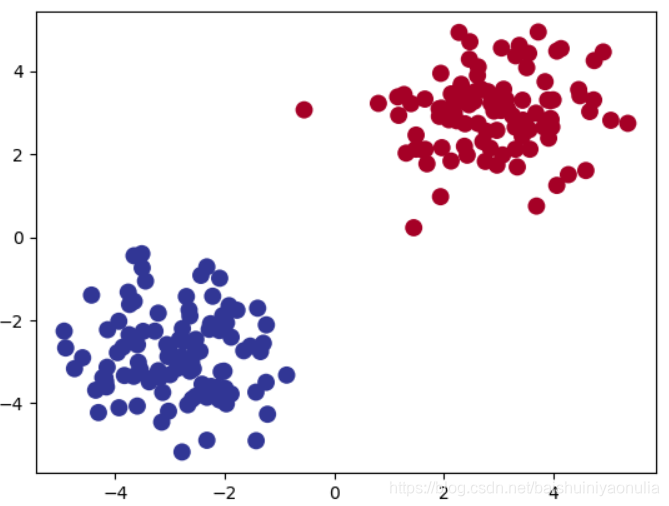
4.1. 分类神经网络

import torch
import torch.nn.functional as F
import matplotlib.pyplot as plt

# 构造数据
n_data = torch.ones(100, 2)
x0 = torch.normal(3*n_data, 1)
x1 = torch.normal(-3*n_data, 1)
# 标记为y0=0，y1=1两类标签
y0 = torch.zeros(100)
y1 = torch.ones(100)

# 通过.cat连接数据
x = torch.cat((x0, x1), 0).type(torch.float)
y = torch.cat((y0, y1), 0).type(torch.long)

# 构造一个简单的神经网络
class Net(torch.nn.Module):
    def __init__(self, n_feature, n_hidden, n_output):
        super(Net, self).__init__()
        self.inLayer = torch.nn.Linear(n_feature, n_hidden) # 输入层
        self.hiddenLayer = torch.nn.Linear(n_hidden, n_hidden) # 隐藏层
        self.outLayer = torch.nn.Linear(n_hidden, n_output) # 输出层

    # 前向计算函数，定义完成后会隐式地自动生成反向传播函数
    def forward(self, x):
        x = F.relu(self.hiddenLayer(self.inLayer(x)))
        x = self.outLayer(x)
        return x

net = Net(2, 10, 2) # 初始化一个网络，2个输入层节点，10个隐藏层节点，2个输出层节点
loss_func = torch.nn.CrossEntropyLoss() # 定义交叉熵损失函数
optimizer = torch.optim.SGD(net.parameters(), lr=0.2) # 配置网络优化器

# 将网络模型、损失函数和输入张量迁入GPU
if(torch.cuda.is_available()):
    net = net.cuda()
    loss_func = loss_func.cuda()
    x, y = x.cuda(), y.cuda()

# 训练模型
out = net(x)
for t in range(300):
    out = net(x) # 将数据输入网络，得到输出
    loss = loss_func(out, y) # 得到损失
    optimizer.zero_grad() # 梯度初始化
    loss.backward() # 反向传播
    optimizer.step() # 对网络进行优化

# 使用模型进行预测
prediction = torch.max(F.softmax(out, dim=0), 1)[1]
pred_y = prediction.data.cpu().numpy().squeeze()

# 可视化
plt.scatter(x.data.cpu().numpy()[:, 0], x.data.cpu().numpy()[:, 1], c=pred_y, s=100, lw=0, cmap='RdYlBu')
plt.show()

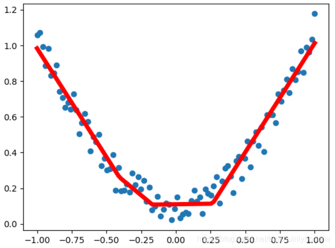
4.2. 回归神经网络

import torch
import torch.nn.functional as F
import matplotlib.pyplot as plt

# 构造数据
x = torch.unsqueeze(torch.linspace(-1, 1, 100), dim=1)
y = x.pow(2) + 0.2 * torch.rand(x.size())

# 构造一个简单的神经网络
class Net(torch.nn.Module):
    def __init__(self, n_feature, n_hidden, n_output):
        super(Net, self).__init__()
        self.inLayer = torch.nn.Linear(n_feature, n_hidden) # 输入层
        self.hiddenLayer = torch.nn.Linear(n_hidden, n_hidden) # 隐藏层
        self.outLayer = torch.nn.Linear(n_hidden, n_output) # 输出层

    # 前向计算函数，定义完成后会隐式地自动生成反向传播函数
    def forward(self, x):
        x = F.relu(self.hiddenLayer(self.inLayer(x)))
        x = self.outLayer(x)
        return x

net = Net(1, 10, 1) # 初始化一个网络，1个输入层节点，10个隐藏层节点，1个输出层节点
loss_func = torch.nn.MSELoss() # 定义均方误差损失函数
optimizer = torch.optim.SGD(net.parameters(), lr=0.2) # 配置网络优化器

# 将网络模型、损失函数和输入张量迁入GPU
if(torch.cuda.is_available()):
    net = net.cuda()
    loss_func = loss_func.cuda()
    x, y = x.cuda(), y.cuda()

# 训练模型
out = net(x)
for t in range(300):
    out = net(x) # 将数据输入网络，得到输出
    loss = loss_func(out, y) # 得到损失
    optimizer.zero_grad() # 梯度初始化
    loss.backward() # 反向传播
    optimizer.step() # 对网络进行优化

# 可视化
plt.scatter(x.data.cpu().numpy(), y.data.cpu().numpy())
plt.plot(x.data.cpu().numpy(), out.data.cpu().numpy(), 'r-', lw=5)
plt.show()

4.3. 多分类神经网络

import numpy as np
import sys
import torch.nn.functional as F
import torch.utils.data as Data
import torch
import matplotlib.pyplot as plt

sys.path.append('./')

# 构造一个简单的神经网络
class Net(torch.nn.Module):
    def __init__(self, n_feature, n_hidden, n_output):
        super(Net, self).__init__()
        self.inLayer = torch.nn.Linear(n_feature, n_hidden) # 输入层
        self.hiddenLayer = torch.nn.Linear(n_hidden, n_hidden) # 隐藏层
        self.outLayer = torch.nn.Linear(n_hidden, n_output) # 输出层

    # 前向计算函数，定义完成后会隐式地自动生成反向传播函数
    def forward(self, x):
        x = self.inLayer(x)
        x = F.relu(self.hiddenLayer(x))
        x = self.outLayer(x)
        return x

# 读取本地数据文件
def loadData(path):
    # delimiter用于设置分隔符，如果是CSV文件那么 delimiter=','
    dataset_df = np.loadtxt(path, dtype=int, delimiter=' ')
    return dataset_df

def show_curve(ys, title):
    '''
    画图
    :param ys: 损失或F1值数据
    :param title: 标题
    :return:
    '''
    x = np.array(range(len(ys)))
    y = np.array(ys)
    plt.plot(x, y, c='b')
    plt.axis()
    plt.title('{} curve'.format(title))
    plt.xlabel('epoch')
    plt.ylabel('{}'.format(title))
    plt.show()
    plt.savefig(fname= title + ".png", dpi=600)
    plt.savefig(fname=title + ".png")
    plt.clf()

def fit(model, loss_func, data_loader, test_data_loader, num_epochs, optimizer):
    """
    进行训练和测试，训练结束后显示损失和准确曲线，并保存模型
    参数:
        model: CNN 网络
        num_epochs: 训练epochs数量
        optimizer: 损失函数优化器
    """

    losses = []
    f1s = []
    for epoch in range(num_epochs):
        print('Epoch {}/{}:'.format(epoch + 1, num_epochs))
        # 训练
        loss = train(model, data_loader, loss_func, optimizer)
        losses.append(loss)

        # 验证
        # 加载模型
        # model = torch.load('./my_net.pth')
        F1 = evaluate(model, test_data_loader)
        f1s.append(F1)
        print("------ Epoch END ------")

    # 损失函数曲线和准确率曲线
    show_curve(losses, "train loss")
    show_curve(f1s, "validation F1")

def train(model, train_loader, loss_func, optimizer):
    """
    训练模块
    model: CNN 网络
    train_loader: 训练数据的Dataloader
    loss_func: 损失函数
    device: 训练所用的设备
    """
    total_loss = 0
    model.train() # 切换至训练模式
    # 批次训练
    for i, (data_tensor, labels) in enumerate(train_loader):
        # 前向传播
        outputs = model(data_tensor)
        loss = loss_func(outputs, labels)

        # 反向传播和优化
        optimizer.zero_grad()
        loss.backward(retain_graph=True)
        optimizer.step()

        total_loss += loss.item()

    # 输出总loss
    print("Train Loss: {:.4f}".format(total_loss))
    return total_loss

def evaluate(model, test_data_loader):
    """
    测试模块，这里使用test代替validation
    model: CNN 网络
    val_loader: 验证集的Dataloader
    device: 训练所用的设备
    return：准确率
    """
    # # 切换至评估模式
    model.eval()
    with torch.no_grad():
        TP = 0 # 预测正确的正样本(1->1)
        FP = 0 # 预测错误的正样本(0->1)
        FN = 0 # 预测错误的负样本(1->0)

        for i, (data_tensor, labels) in enumerate(test_data_loader):
            outputs = model(data_tensor)
            # 选取最大输出值的类别进行分类
            _, predicted = torch.max(outputs.data, dim=1)

            # 根据几个类别的输出值赋予相对应的概率,然后根据概率值进行分类
            # _ = F.softmax(outputs.data, dim=1)
            # predicted = Categorical(_).sample()

            # 输出神经网络的预测值与实际label，比较预测结果
            # print(str(i+1) + " Predicted: " + str(predicted))
            # print(str(i+1) + " Label: " + str(labels))

            for j in range(len(predicted)):
                if (labels[j] == 1) and (predicted[j] == labels[j]):
                    TP += 1
                if (labels[j] == 1) and (predicted[j] != labels[j]):
                    FN += 1
                if (labels[j] == 0) and (predicted[j] != labels[j]):
                    FP += 1

        if (TP + FP) == 0: # 精确率
            precision = 0
        else:
            precision = TP / (TP + FP)
        if (TP + FN) == 0: # 召回率
            recall = 0
        else:
            recall = TP / (TP + FN)
        if (precision + recall) == 0: # F1
            F1 = 0
        else:
            F1 = (2 * precision * recall) / (precision + recall)

        print('Precision on Test Set: {:.4f} %'.format(100 * precision))
        print('Recall on Test Set: {:.4f} %'.format(100 * recall))
        print('F1 on Test Set: {:.4f} %'.format(100 * F1))

        return F1

if __name__ == "__main__":
    # ------ 构造训练数据 ------ #
    n_data = torch.ones(1000, 2) # 1000行2列的矩阵，即1000个二维坐标点
    x0 = torch.normal(3 * n_data, 1) # 给原二维坐标点加正太扰动，x0在第一象限
    x1 = torch.normal(-3 * n_data, 1) # 给原二维坐标点加正太扰动，x1在第三象限
    x = x0 + x1 # 拼接数据

    # 构造label，标记为y0=0，y1=1两类标签
    y0 = torch.zeros(1000) # 1000个0
    y1 = torch.ones(1000) # 1000个1
    y = y0 + y1 # 拼接数据

    # ------ 将数据载入DataLoader ------ #
    x_tensor = torch.Tensor(x).type(torch.float)
    y_tensor = torch.Tensor(y).type(torch.long)  # label不能是浮点数

    torch_dataset = Data.TensorDataset(x_tensor, y_tensor)
    data_loader = Data.DataLoader(  # 训练数据
        dataset=torch_dataset,
        batch_size=32,  # 从torch_dataset中每次抽出batch size个样本
        shuffle=True  # 随机排序
    )

    # 构建测试数据加载器(data+label)
    torch_test_dataset = Data.TensorDataset(x_tensor, y_tensor)
    test_data_loader = Data.DataLoader(  # 测试数据
        dataset=torch_dataset,
        batch_size=len(torch_test_dataset),  # 从torch_dataset中每次抽出全部样本
        shuffle=False  # 不随机排序
    )

    # ------ 网络参数定义 ------ #
    # 输入数据的维度即输入层的维度，这里是2，因为坐标点是二维的
    input_layer_size = len(x[0])
    # 初始化一个网络，input_layer_size个输入层节点，256个隐藏层节点，
    # 2个输出层节点（因为是2分类任务，n个分类输出层节点个数就是n）
    CNN_model = Net(input_layer_size, 256, 2)
    loss_func = torch.nn.CrossEntropyLoss() # 损失函数，这里是交叉熵损失，可以换用其他的损失函数
    optimizer = torch.optim.SGD(CNN_model.parameters(), lr=0.01, momentum=0.9)  # 配置网络优化器

    # 训练设备，有GPU就用GPU，没就用CPU
    if (torch.cuda.is_available()):
        print("Using CUDA")
        mgcnn = CNN_model.cuda()
        loss_func = loss_func.cuda()
        x_tensor = x_tensor.cuda()
        y_tensor = y_tensor.cuda()

    # 开始训练
    epochs = 100 # 训练轮数
    fit(CNN_model, loss_func, data_loader, test_data_loader, epochs, optimizer)
    torch.save(CNN_model, './my_net.pth') # 保存模型