使用logistic regression 多分类预测

逻辑回归（logistic regression）可以用来进行分类预测，一般进行两个类别的预测，因为逻辑回归预测输出仅为0和1.

逻辑回归也可以预测多个分类。可以使用如下技巧：

1）假设类别K个

2）将数据集中类别i(i<=k)对应的标签lable标记为1，其余类别标记为0，使用逻辑回归训练出一组对应参数theta值

3）使用2，重复k次，训练处k组theta。预测时，分别使用k组theta预测数据x，可出k个预测结果，选出最大预测值对应的那组theta

4）选出3中得到的theta对应的类别i，so,i就是预测出的类别。

下面使用逻辑回归学习算法预测10个数字，数字使用图片表示，每张图片由20*20个像素组成，代表一个数字。一共有5000个数字，所以在文件ex3data1.mat中有5000*400这样一个矩阵，5000代表5000个数据，400代表每个数据的20*20个像素。ex3data1.mat中还有一个长度为5000的向量，是对应5000个数据的标签，也就是该行数据代表的数字。

好，先选出100个数据，使用2-D图表示看一下：

def displayData(X, theta=None):
    width = 20
    rows, cols = 10, 10
    out = zeros(( width * rows, width * cols ))

    rand_indices = random.permutation(5000)[0:rows * cols]

    counter = 0
    for y in range(0, rows):
        for x in range(0, cols):
            start_x = x * width
            start_y = y * width
            out[start_x:start_x + width, start_y:start_y + width] = X[rand_indices[counter]].reshape(width, width).T
            counter += 1

    img = scipy.misc.toimage(out)
    figure = pyplot.figure()
    axes = figure.add_subplot(111)
    axes.imshow(img)

    if theta is not None:
        result_matrix = []
        X_biased = c_[ones(shape(X)[0]), X]

        for idx in rand_indices:
            result = (argmax(theta.T.dot(X_biased[idx])) + 1) % 10
            result_matrix.append(result)

        result_matrix = array(result_matrix).reshape(rows, cols).transpose()
        print result_matrix

    pyplot.show()

加载数据，调用上面这个display函数：

    mat = scipy.io.loadmat("ex3data1.mat")
    X, y = mat['X'], mat['y']
    displayData(X)

显示效果：

下面一步一步实现logistic regression：

1）写sigmoid函数（详细解释看http://blog.csdn.net/bdss58/article/details/41983463）：

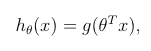
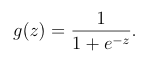
def sigmoid(z):
    return 1.0 / (1.0 + exp(-z))

2）计算代价函数：

def computeCost(theta, X, y, lamda):
    m = shape(X)[0]
    hypo = sigmoid(X.dot(theta))
    term1 = log(hypo).dot(-y)
    term2 = log(1.0 - hypo).dot(1 - y)
    left_hand = (term1 - term2) / m
    right_hand = theta.T.dot(theta) * lamda / (2 * m)
    return left_hand + right_hand

3） 计算梯度：

def gradientCost(theta, X, y, lamda):
    m = shape(X)[0]
    grad = X.T.dot(sigmoid(X.dot(theta)) - y) / m
    grad[1:] = grad[1:] + ( (theta[1:] * lamda ) / m )
    return grad

4）训练出K组theta，这里有10个数字，所以k=10:

def oneVsAll(X, y, num_classes, lamda):
    m, n = shape(X)
    X = c_[ones((m, 1)), X]
    all_theta = zeros((n + 1, num_classes))

    for k in range(0, num_classes):
        theta = zeros(( n + 1, 1 )).reshape(-1)
        temp_y = ((y == (k + 1)) + 0).reshape(-1)
        result = scipy.optimize.fmin_cg(computeCost, fprime=gradientCost, x0=theta, \
                                        args=(X, temp_y, lamda), maxiter=50, disp=False, full_output=True)
        all_theta[:, k] = result[0]
        print "%d Cost: %.5f" % (k + 1, result[1])
    return all_theta

5）预测

def predictOneVsAll(theta, X, y):
    m, n = shape(X)
    X = c_[ones((m, 1)), X]

    correct = 0
    for i in range(0, m):
        prediction = argmax(theta.T.dot(X[i])) + 1
        actual = y[i]
        # print "prediction = %d actual = %d" % (prediction, actual)
        if actual == prediction:
            correct += 1
    print "Accuracy: %.2f%%" % (correct * 100.0 / m )