SVD&Search Engines

An Introduction to Singular Value Decomposition

What Does This Have to do With Search Engines?

So, to review, in order to run a search engine with the vector space model, we first have to convert the entire world wide web into a term-by-document matrix. This matrix would be huge! It would have to be at least 300,000 x 3,000,000,000 according to the most conservative estimates. Processing a query for this kind of vector space would be ridiculous. We would have to find the angle measures between the query vector and billions of other 300,000 dimensional vectors for every query! That would take way too long for practical purposes. Fortunately, there are some tricks in linear algebra that we can use to cut a few corners.

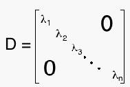
You may remember from your linear algebra class that Eigen Decomposition can make many calculations much quicker and easier. For example, suppose we have a matrix A, and we want to find A³. Instead of computing A*A*A, which could require a lot of calculation (especially if A is large), we can use the eigen decomposition A=P*D*P^-1; where
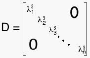
and λ1...λn are the eigenvalues of A. Now A=P*D³*P^-1, or
which is much easier to calculate. Since this method of decomposition can only be used on square matrices, we have no use for it. BUT we can use Singular Value Decomposition, which works in much the same way.

What's so Special about SVD?

Singular Value Decomposition has two wonderful properties that make it very helpful and important for our work. First, it exists for any and all matrices: large, small, square, rectangular, singular, non-singular, sparse and dense. So, no matter what kind of term by document matrix the internet yields, we know it has a singular value decomposition.

The next helpful property is the optimality property. This property basically tells us that, if we would like to find a rank-k approximation of our matrix, the best one can be found using singular value decomposition. I will explain this property in more detail a little bit later on in your training.

So What is Singular Value Decomposition?

Definition: Given that an mxn matrix A has rank r, A can be factored where U and V are orthogonal matrices containing the singular vectors, and S is a matrix of the form where D is a diagonal matrix containing the singular values of A.

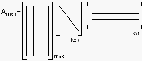
So, basically, SVD breaks A into three components:

It would probably help your understanding of SVD if we actually look at some examples. With the help of MATLAB, we can easily calculate and compare the SVDs of a few matrices. If you are not familiar with MATLAB, you may want to read through this tutorial.

Activity 3

In the following and later activities we will be using some of the m-files from the ATLAST project. To download these, go to the ATLAST page and download the m-files for the second edition (pay attention to where the computer puts them).

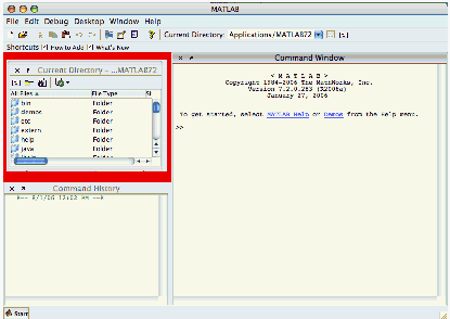
Now open MATLAB. We need to have the ATLAST files open in the current directory.

The location of the folder will be different depending on what kind of computer you are working with. Find it by navigating through the directory and selecting the atlast65 folder as shown above.

Create a random 5 by 6 matrix of rank 4 and entries between 2 and -2 with the command:
A = randintr(5,6,2,4)
(Learn more about this command; enter help randintr)

Find the singular value decomposition of your matrix A by typing[U,S,V] = svd(A)
This command calculates the svd and allows you to see each component of the decomposition.

How many singular values does A have?

Try the same thing with A = randintr(5,6,2,5). Now how many singular values does A have? Can you see a relationship between the rank of a matrix and how many singular values it has?

It just so happens that, if r is the rank of A, then r is also the number of non-zero entries of S (in other words, r is the number of singular values of A). Berry & Brown

Now that we know what SVD, we can look more closely at how it can help our search engine by making the calculations a bit less arduous.

Truncated SVD and its Applications

What is a truncated SVD?

On the previous page, we learned that singular value decomposition breaks any matrix A down so that A = U*S*V'. Let's take a closer look at the matrix S.

Remember S is a matrix of the form where D is a diagonal matrix containing the singular values. D, as one might guess, looks like this: where are the singular values of the matrix A with rank r. A full rank decomposition of A is usually denoted like this: .

We can find a reduced rank approximation (or truncated SVD) to A by setting all but the first k largest singular values equal to zero and using only the first k columns of U and V.

The Optimality Property

Why are we using this particular decomposition for our rank k approximations? According to the optimality property, singular value decomposition gives the closest rank k approximation of a matrix. What do I mean by close?

A theorem proven by Eckart and Young shows that the error in approximating a matrix A by Ak can be written:

where B is any matrix with rank k. The notation on the left means that we are taking the Frobenius norm of the matrix A-A k. You may remember finding the length or magnitude of a vector as a way of measuring its size. The Frobenius norm does much the same thing except with entire matrices. So, this formula means tells us that the difference between A and A k is smaller than the difference between A and any other rank k matrix B. We cannot find or even make up another matrix of rank k that will be closer to A.

Choosing a k

So what k should we choose? If we choose a higher k, we get a closer approximation to A. On the other hand, choosing a smaller k will save us more work. Basically, we must choose between time and accuracy. Which do you think is more important? How can we find a good balance between sacrificing time and sacrificing data?

Activity 4

One trick is to look at and compare all the singular values of your matrix. Create a random matrix A in MATLAB using the randintr command we used earlier. Now calculate only the singular values of your matrix with the command
svd(A).
Now plot these values by entering
plot(svd(A)).
Note how the singular values decrease. When we multiply U, S, and V back together, the larger singular values contribute more to the magnitude of A than the smaller ones. Are any of the singular values of your matrix A significantly larger than the others?

Now create the following matrix N in MATLAB:

Again calculate the singular values (rather than the whole decomposition) and plot the values. Are any of the singular values for this matrix significantly higher than the others? What do you think we should choose as our k for this matrix?

Comparing Rank-k approximations

We can also look at the approximations themselves to help us decide which k to use. Sometimes, we can get a good idea of how close an approximation is by looking at the matrices themselves, but this would only be practical for very small matrices. In most cases, it helps to use a graph to represent the matrix.

Activity 5

Download the following m-files for the following MATLAB activity.

cityplot.m
displaySVD2.m

Do you still have your term-by-employee matrix stored? If not, re-enter it into MATLAB and store it as matrix A (or another variable you prefer).

Drag the files into the current directory and enter the command
displaySVD2(A)

A window should pop-up showing two "city plot" graphs: one of the rank 1 approximation of your matrix and one of the matrix itself. The graphs should look something like this:

To find the value of each entry, match the colors of the tops of each "building" with the values on the color bar to the right of each graph.

Look at each graph from different angles by clicking on the "rotate" icon at the top of the window, then clicking and dragging the graph around.

When you're done looking at these two graphs, hit the space bar and the rank 2 approximation will appear. Continue to examine and compare the graphs until you have seen all k approximations.

If you had to choose a k based on these graphs, which would you choose? Why? What do your co-workers think?

Hopefully this exercise gave you a better idea of what the rank k approximations look like as k gets closer and closer to r (or the rank of the original matrix).

SVD has been useful in many other fields outside of information retrieval. One example is in digital imaging. It turns out that when computers store images, they store them as giant matrices! Each numerical entry of a matrix represents a color...sort of like a giant paint-by-number. How could SVD be useful here?

Activity 6

Make sure the ATLAST commands are in your current directory again, then enter the commands:
load gatlin2
image(X), colormap(map)
This will create a 176x260 matrix X representing the image you see after entering the second command.

Now enter ATLAST command svdimage(X,1,map)and a new window containing two images should appear. The one on the left is the original image, and the one on the right is a rank 1 approximation of that image. Hit any key and the rank increases by one.

What would be a good k for your image? How much storage space would the computer save by storing this approximation in decomposed form (mxn numbers to store for the original matrix vs. mxk + k + nxk numbers to store for the decomposed rank k approximation)?

For completely dense matrices, like images, we can obviously save a lot on storage. Would we save a lot on storage for a sparser matrix like our term-by-document matrices?

Computers store sparse matrices in a different way; they only store the non-zero entries of the matrix. Storage savings is probably not going to be our motivation for using rank-k approximations. So why do we use it?

Calculating a Query with SVD

As you may recall, the equation for calculating the cosine of the angle between a query vector and another vector is:

Since A ke j equals the jth column of the rank k matrix A, then we can rewrite the formula:

where the vector A ke j is simply the jth column of the rank-k matrix A k. Now if we write A k in terms of its singular value decomposition, we have:

If we let s j= then we can simplify the formula to:

for j= 1, 2, 3, 4, ...n. The vectors s j and norms || s j|| 2 only need to be computed once, then they can be stored and retrieved when a query is being processed. So now, all that has to be computed at query time is ||q|| 2 and Berry & Brown, 1999. This is still a bit of an expensive calculation, but not nearly as expensive as processing a query without SVD.

Where Else is This Being Used?

Not many search engines are still using the vector space model and SVD to process queries. Is Company Enterprises the only company still taking advantage of this method? Not completely. Some companies are still using Latent Semantic Indexing (LSI) which is a method that uses SVD. According to Langville, 2005,

		the LSI method manipulates the matrix to eradicate 
		dependencies and thus consider only the independent, 
		smaller part of this large term-by-document matrix. 
		In particular, the mathematical tool used to achieve the 
		reduction is the truncated singular value decomposition 
		(SVD) of the matrix. 

Here's an example of how a company is using LSI to its advantage.

Congratulations! You have now learned all you need to know about the vector space model and singular value decomposition and so have completed your training for Company Enterprises. Continue on to the next page for your first assignment as an official employee of Company Enterprises.

A Quick Look at How Search Engines Work

File Preparation

Before a search engine can retrieve any documents, they have to be organized. Libraries have to go through all their books and systematically organize them to make them easy for readers to find, and search engines must do something similar.

Of course, this task proves a bit difficult because of the heterogeneity of web pages. Should the page be organized according to its title or its content? How much of the content should be considered? Should pictures be considered or disregarded?

This is called indexing. Some engines do this manually (which means they pay lots and lots of people to sit at computers and index as many pages as they can...which is not very many). Since this is an obviously expensive (both in time and money) method, most engines opt for automatic indexing by using web crawlers.

These are computer programs that "crawl" the web, pull up webpages, consider the content, and index the page. Web crawlers can index from 3 to 10 million pages per day. Unfortunately, automatic indexing is not nearly as accurate as manual indexing. For example, webmasters can easily trick many web crawlers by inserting popular search words such as "football" or "movies" into the page and making them the same color as the background (this is referred to as spamming)Berry & Brown.

Retrieving Information

Once the web pages have been indexed, the engine can go back and retrieve them in response to a query from a user, similar to a reader searching a card catalog in a library.

Several different types of search engines have been created so far, each with their advantages and disadvantages. The following table provides a quick overview of these different types:

Type of Search Engine	Description	Advantages	Disadvantages
Boolean	Uses Connectors (and, or, not)	Easy to use Queries processed quickly Complexity doesn't increase with size	No partial matches Synonymy Polysemy
Probabilistic Model	Underlying algorithm guesses at relevance	Pages ranked by odds of relevance to user	Very hard to build Complexity grows quickly
Vector Space Model	Uses linear algebra to find connections in document collection	Reveals semantic meaning Opportunity for feedback	High computational expense

The benefits of the vector space model (VSM) far outweigh its computational expense. This is why Company Enterprises has decided to build a search engine based on VSM, and why the remainder of your training will focus on this model.

A Closer Look at the Vector Space Model

Preparing the Documents

Before VSM can be used to process any queries, all documents must be prepared. A giant term by document matrix is created where the columns represent web documents and the rows represent terms. If a document contains a term, the corresponding row of that vector will have a 1, otherwise there will be a 0.

For example, lets look at the survey you took earlier. We can use the information in your survey to create a "term-by-employee" vector by placeing a 1 next to the terms you selected and a 0 next to the terms you did not select.

Coffee	(0 or 1)
Tea	(0 or 1)
Donuts	(0 or 1)
Muffins	(0 or 1)
Morning	(0 or 1)
Evening	(0 or 1)
Monday	(0 or 1)
Tuesday	(0 or 1)
Wednesday	(0 or 1)
Thursday	(0 or 1)
Friday	(0 or 1)
12:00	(0 or 1)
1:00	(0 or 1)
Kickball	(0 or 1)
Trivia	(0 or 1)

Combine your vector with those of the other employees around you to create a term-by-employee matrix, much, much smaller but very similar to the term-by-document matrix representing the entire World Wide Web.

So why is it useful to convert the web into a matrix? Well, it just so happens that mathematicians know a great deal about the properties of matrices, and so we can use this knowledge to learn the properties of the world wide web.

Processing a Query

When a user enters a query in the search engine, the computer converts the query into a vector the same way it converted the web documents. Then it uses linear algebra to find the document closest to the vector.

Activity 2.1

To help better understand how it does this, lets look at our term-by-employee matrix again, and in order to get a better visual of the process let's only consider the vector space created by the Coffee, 12:00, and Kickball rows of the matrix.

Since our matrix now only has three dimensions, we can plot each employee's vector in a 3-dimensional space. Let Coffee be the X-axis, 12:00 be the Y-axis, and Kickball be the Z-axis. Fold a piece of graph paper as shown:

1. Make sure the piece of paper is square and cut along the red line as shown.
2. Fold the square in half twice to form a horizontal and vertical crease through the middle, then cut along the red line as shown.
3. Align flaps so that one is on top of the other (it doesn't matter which) as shown.
4. Now you should have a cube-like structure made out of graph paper representing the non-negative quadrant of R³. Label your X, Y, and Z axes.

Now that you have your 3-D graph, use pipe-cleaners to graph each of the vectors representing employees.

What if you were a employee who enjoys coffee and kickball, and you would like to find a co-worker who shares your interests. Create a 3-dimensional query vector representing a query for Coffee and Kickball (so the vector should be [1 0 1]). Which employee do you think is the closest match? Is the answer obvious? Try other queries.

This method, though it may seem good enough for now, is not quite precise enough for our liking, and is also impossible once we move into four or more dimensions. So let's look at a more mathematical method.

Any vector can be summarized by its length and its angle relative to another fixed vector. Once we know the length of two vectors x and y, we can easily find the cosine of the angle between them with the following formula:

If the vectors are parallel (they are very related), the cosine of their angle will be 1. If the vectors are orthogonal (they are unrelated), the cosine of their angle will be 0.

Find the cosines of the angles between all of the employee vectors and two or three of your query vectors. Which employees best match the query? Were your guesses correct?

One of the main advantages of the Vector Space Model is that we can make it more complex without greatly complicating the calculations. For example, the method works as well in millions of dimensions as it did in our tiny three dimension example (though the calculations would take considerably longer).

Of course, once we start working with millions of terms and millions of documents, it may become harder to discern which documents should be considered relevant. One solution to this problem is to add weights to terms when indexing. There are several ways to weight the terms in a document, but one very good example is to weight the terms by percentage of relevance.

For example, say you were indexing a garden article that talked about the different fertilizers that mentioned special types of fertilizers for gardenias and roses. We would certainly want to signify "fertilizer," rose," and "gardenia" as important terms for the document, but assigning the vector: misrepresents the document. The term "fertilizer" should certainly carry more weight. Instead we might want a vector that looked more like: . This vector tells us that 80 percent of the article pertains to fertilizer, while only 10 percent pertains to both roses and gardenias. This is certainly a much more accurate representation our document.

When working with such a large number of documents, we might also face a problem of too many documents being returned to answer a query. This could be daunting for a hapless searcher, but also wastes time for the search engine. A cut-off point seems appropriate. Luckily for us this is not hard to execute with the VSM.

To set our cut-off value, we can simply tell our search engine not to return any documents whose angle with the query is greater than, say, 45 degrees (or cosine values less than .7071). If we were to make an image of this 45 degree cut-off, it would look something like this:

	
			
				(image from Langville)

Activity 2.2

To get a better idea of what a cut-off would look like in three dimensions, take another piece of paper and create a cut-off cone for the coffee and kickball query in the three-dimensional term-by-employee vector space. First make a cone for the 45 degree cut-off (like in the picture shown above). Are any employees cut-off? Now make 30 degree and 15 degree cut-off cones and compare the results with the first one. Are these cut-offs useful?

Flaws of the Vector Space Model

What more could we want in a search engine? The Vector Space Model seems like a watertight method so far. True, the VSM seems to be the best search engine model we have seen so far, but it is far from perfect.

Since there are more than 3 billion documents on the web, a search engine using the vector space model would have to calculate more than 3 billion angle measures for every single query. Then of course all of the documents returned (and aren't cut-off) must be ranked for the user. And ideally this should all happen in less than a second. This of course is not possible. So what can we do?

Luckily we have been saved from our plight by the process of singular value decomposition. So, we should probably take some time to learn all about this powerful tool.

转：http://langvillea.people.cofc.edu/DISSECTION-LAB/Emmie%27sLSI-SVDModule/p3module.html

---

---