禁忌搜索算法完整指南（python）

这次我们要聊的是——禁忌搜索算法。相信不少小伙伴在面对复杂问题时，常常会陷入局部最优解的困境，而禁忌搜索算法能帮助我们有效避免这种情况，找到更优的解决方案。废话不多说，让我们直接进入正题。

一、禁忌搜索算法简介

（一）引言

在实际生活中，很多问题都可以转化为优化问题，比如生产调度、物流配送、旅行商问题等等。对于这些问题，我们需要找到一个最优解或者接近最优解的解。然而，传统的一些优化算法，如贪心算法、动态规划等，往往只能找到局部最优解，而不能保证全局最优解。这时候，我们需要一些更强大的算法来帮助我们解决问题，禁忌搜索算法就是其中一种。

（二）算法背景

禁忌搜索算法（Tabu Search，TS）是由美国数学家 Fred Glover 在20世纪80年代提出的一种元启发式搜索算法。它是一种局部搜索的扩展，通过引入禁忌机制来避免陷入局部最优解。禁忌搜索算法的灵感来源于人类的思考过程，当我们遇到问题时，会尝试不同的解决方案，如果某个方案被证明是无效的，我们就会把它标记为禁忌，不再轻易尝试。

（三）算法特点

1. 局部搜索的扩展：禁忌搜索算法基于局部搜索，通过不断地探索邻域来寻找更优的解。但与普通的局部搜索不同，它引入了禁忌表来记录已经被访问过的解或者某些特定的操作，防止算法在搜索过程中反复访问相同的解，从而扩大搜索范围。

2. 禁忌机制：这是禁忌搜索算法的核心机制。禁忌表中记录了最近搜索到的一些解或者移动操作，这些被禁忌的解或操作在一定的时期内（禁忌长度）不能被再次选择，除非满足一定的赦免条件，如发现更好的解。

3. 灵活性和自适应性：禁忌搜索算法具有很强的灵活性和自适应性，可以通过调整禁忌表的大小、禁忌长度、候选解的生成方式等参数来适应不同的问题和搜索需求。

4. 全局搜索能力：通过禁忌机制，禁忌搜索算法能够在更大的搜索空间中探索，从而提高找到全局最优解的可能性。

二、禁忌搜索算法的基本原理

（一）基本概念

1. 邻域：在禁忌搜索算法中，邻域是指当前解周围的一组解，这些解可以通过一些简单的变换得到。例如，在旅行商问题中，一个解的邻域可以包括通过交换两个城市的位置得到的所有解。

2. 禁忌表 ：禁忌表是一个记录表，用于存储已经被访问过的解或者移动操作。禁忌表的大小和管理方式对算法的性能有很大的影响。禁忌表通常是一个列表，存储的内容可以是解、移动操作或者其他特征，具体取决于问题的性质。

3. 候选解 ：在每次迭代中，算法会从邻域中选择若干个候选解进行评估。候选解的选择方式可以是随机的，也可以是基于某些启发式规则。

4. 评价函数 ：评价函数用于评估解的质量。对于不同的问题，评价函数的定义也不同。例如，在旅行商问题中，评价函数可以是旅行的总距离；在生产调度问题中，评价函数可以是生产周期。

（二）算法步骤

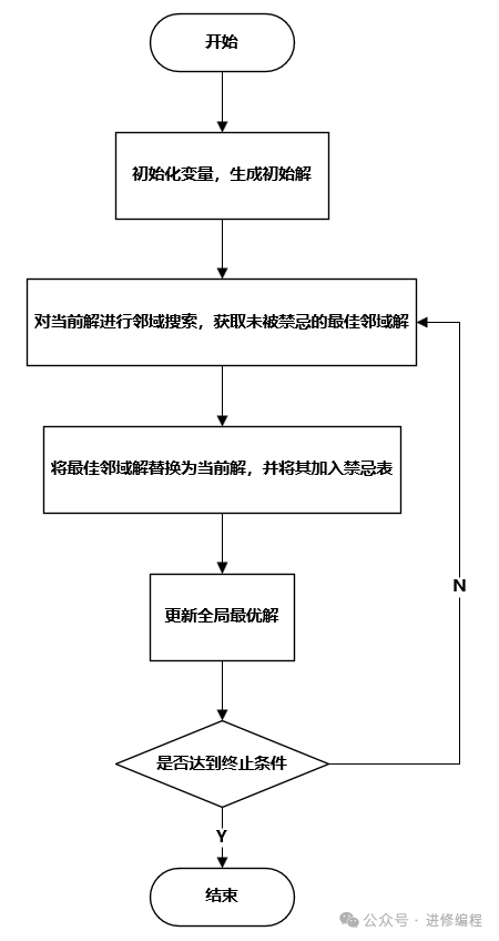
禁忌搜索算法的基本步骤如下：

1. 初始化 ：随机生成一个初始解作为当前解，并设置禁忌表为空。

2. 生成邻域 ：根据当前解生成一组邻域解。

3. 选择候选解 ：从邻域解中选择一组候选解。

4. 评估候选解 ：使用评价函数对候选解进行评估。

5. 选择最优解 ：从候选解中选择最优解作为下一个当前解。如果该解不在禁忌表中，或者满足某些赦免条件（如该解优于当前找到的最优解），则将其作为新的当前解。

6. 更新禁忌表 ：将当前选择的移动操作或解添加到禁忌表中，并根据禁忌长度和规约策略更新禁忌表。

7. 终止条件判断 ：如果满足终止条件（如达到最大迭代次数、找到满意的解等），则停止算法，输出最优解；否则，返回步骤2继续搜索。

（三）禁忌表的管理

禁忌表的管理是禁忌搜索算法中的一个关键环节。禁忌表的大小通常是一个相对较小的正整数，用于控制搜索过程中记忆的长度。禁忌表的管理策略包括：

1. 禁忌长度 ：禁忌长度决定了一个解或移动操作在禁忌表中停留的时间。通常，禁忌长度可以是一个固定值，也可以是动态调整的。例如，可以将其设置为邻域大小的20%。

2. 规约策略 ：当禁忌表的大小超过一定限制时，需要采用规约策略来删除一些较旧的解或移动操作。常见的规约策略包括先进先出（FIFO）、最不常使用（LFU）等。

3. 赦免条件 ：尽管某个解或移动操作在禁忌表中，但如果它满足某些特定的条件，如当前解优于全局最优解，它可以被赦免，从而被选为新的当前解。

三、真实案例：使用Solomon标准数据集解决VRP

为更好地理解如何应用禁忌搜索算法解决VRP，我们将使用Solomon标准数据集中的一个实例。Solomon数据集是VRP研究领域广泛使用的基准数据集，包含了多种不同类型的VRP实例，适用于各种算法和模型的测试与评估。 

1. 初始化

禁忌搜索的第一步是初始化一个“当前解”，这个解通常是一个随机解。然后，通过计算当前解的目标函数（如路径总长度）来设定初始的最优解。

在代码中：

current_path = list(range(n))random.shuffle(current_path)  # 随机初始化路径best_path = current_path[:]  # 复制当前路径作为初始最优路径best_length = path_length(best_path, customers)  # 计算路径长度

我们随机初始化了一个路径（客户的访问顺序），并计算该路径的总长度（目标函数值）。然后，初始路径和长度分别作为当前路径和最优路径。

2. 生成邻域解

禁忌搜索的核心思想是不断从当前解的“邻域”中生成新的解，并通过评估目标函数来选择最优的邻域解。邻域解是通过对当前解进行一定程度的“扰动”生成的。例如，可以通过交换路径中的两个客户来生成邻域解。

在代码中，邻域解是通过交换路径中两个客户的位置来生成的：neighborhood = []

for i in range(n):    for j in range(i + 1, n):  # 对路径中的每一对客户进行交换        if tabu_list[i, j] == 0:  # 检查该交换是否在禁忌表中            neighbor = current_path[:]  # 复制当前路径            neighbor[i], neighbor[j] = neighbor[j], neighbor[i]  # 交换客户            neighborhood.append((neighbor, i, j))

此处，我们遍历路径中的每一对客户，通过交换它们的位置来生成新的邻域解。如果交换的路径不在禁忌表中（即未被禁止的解），我们就将其加入邻域列表。

3. 选择最优邻域解

从生成的邻域解中，选择一个具有最佳目标函数值（最短路径）的解。这是禁忌搜索算法的一部分，它确保算法能在当前的局部区域内寻找最优解。

在代码中：​​​​​​​

best_neighbor = Nonebest_neighbor_length = float('inf')
for neighbor, i, j in neighborhood:    length = path_length(neighbor, customers)  # 计算路径长度    if length < best_neighbor_length:        best_neighbor_length = length  # 更新最优解        best_neighbor = (neighbor, i, j)

我们遍历所有邻域解，选择一个路径总长度最小的解作为当前最优邻域解。

4. 更新禁忌表

禁忌搜索的关键在于禁忌表，它用于记录当前解中的某些操作（如交换的客户），以避免搜索过程中返回到之前的解。禁忌表可以防止搜索陷入局部最优解。

在代码中：​​​​​​​

i, j = best_neighbor[1], best_neighbor[2]tabu_list[i, j] = tabu_tenure  # 将这次交换添加到禁忌表中tabu_list[j, i] = tabu_tenure  # 因为交换是双向的

我们将当前最优邻域解的交换操作（即客户 i 和 j 的交换）加入禁忌表，并设置一个衰退周期（tabu_tenure），这个周期决定了禁忌表中记录的操作持续的时间。

5. 禁忌表衰退

禁忌表不是永久有效的。随着算法的进行，禁忌表中的条目会逐步“衰退”，这意味着禁忌表中的某些条目会在多次迭代后变得无效，从而允许之前的操作再次发生，避免过早停止搜索。

在代码中：

tabu_list[tabu_list > 0] -= 1  # 衰退禁忌表

每次迭代后，禁忌表中的每个值减一，直到它们变为零，表示这些操作不再被禁忌。

6. 终止条件

禁忌搜索会在满足某些终止条件时停止，例如达到最大迭代次数或找到满足要求的解。

在代码中：​​​​​​​

for iteration in range(max_iter):    # 生成邻域解、选择最优解、更新禁忌表等操作

算法将继续进行 max_iter 次迭代。在每一轮迭代中，禁忌搜索会选择邻域中最好的解并更新当前解，直到达到指定的最大迭代次数。

7. 输出最优解

最终，禁忌搜索会输出最优的路径和该路径的总长度。

在代码中：​​​​​​​

print(f"Best Path: {best_path}")print(f"Best Path Length: {best_length:.2f}")

完整代码

import numpy as np
import random
import matplotlib.pyplot as plt
import seaborn as sns

# 设定 Seaborn 样式
sns.set(style="darkgrid")

# 设定 Matplotlib 中文支持（适用于 Windows）
plt.rcParams['font.sans-serif'] = ['SimHei']  # 适用于 Windows（黑体）
plt.rcParams['axes.unicode_minus'] = False  # 解决负号显示问题

# ---------------------------
# 1. 真实数据定义：Berlin52 数据集
# ---------------------------
berlin52_cities = [
    (565, 575), (25, 185), (345, 750), (945, 685), (845, 655), (880, 660), (25, 230),
    (525, 1000), (580, 1175), (650, 1130), (1605, 620), (1220, 580), (1465, 200),
    (1530, 5), (845, 680), (725, 370), (145, 665), (415, 635), (510, 875), (560, 365),
    (300, 465), (520, 585), (480, 415), (835, 625), (975, 580), (1215, 245), (1320, 315),
    (1250, 400), (660, 180), (410, 250), (420, 555), (575, 665), (1150, 1160), (700, 580),
    (685, 595), (685, 610), (770, 610), (795, 645), (720, 635), (760, 650), (475, 960),
    (95, 260), (875, 920), (700, 500), (555, 815), (830, 485), (1170, 65), (830, 610),
    (605, 625), (595, 360), (1340, 725), (1740, 245)
]

# ---------------------------
# 2. 计算城市间的距离矩阵
# ---------------------------
def calculate_distance(city1, city2):
    return np.hypot(city1[0] - city2[0], city1[1] - city2[1])

def create_distance_matrix(cities):
    n = len(cities)
    matrix = np.zeros((n, n))
    for i in range(n):
        for j in range(n):
            matrix[i][j] = calculate_distance(cities[i], cities[j])
    return matrix

# ---------------------------
# 3. 初始解生成（最近邻启发式）
# ---------------------------
def nearest_neighbor_solution(distance_matrix):
    n = len(distance_matrix)
    current = random.randint(0, n - 1)
    solution = [current]
    unvisited = set(range(n))
    unvisited.remove(current)
    
    while unvisited:
        next_city = min(unvisited, key=lambda city: distance_matrix[current][city])
        solution.append(next_city)
        unvisited.remove(next_city)
        current = next_city
    return solution

def route_length(solution, distance_matrix):
    total = sum(distance_matrix[solution[i]][solution[(i + 1) % len(solution)]] for i in range(len(solution)))
    return total

# ---------------------------
# 4. 破坏（Destroy）与修复（Repair）操作
# ---------------------------
def destroy_operator(solution, removal_rate=0.2):
    n = len(solution)
    num_remove = max(1, int(n * removal_rate))
    removed_indices = sorted(random.sample(range(1, n), num_remove))
    removed_nodes = [solution[i] for i in removed_indices]
    partial_solution = [city for i, city in enumerate(solution) if i not in removed_indices]
    return partial_solution, removed_nodes

def repair_operator(partial_solution, removed_nodes, distance_matrix):
    solution = partial_solution.copy()
    for node in removed_nodes:
        best_increase, best_position = float('inf'), None
        for i in range(len(solution)):
            j = (i + 1) % len(solution)
            increase = (distance_matrix[solution[i]][node] + distance_matrix[node][solution[j]] -
                        distance_matrix[solution[i]][solution[j]])
            if increase < best_increase:
                best_increase, best_position = increase, j
        solution.insert(best_position, node)
    return solution

# ---------------------------
# 5. LNS 主算法
# ---------------------------
def LNS_TSP(cities, iterations=1000, removal_rate=0.2):
    distance_matrix = create_distance_matrix(cities)
    current_solution = nearest_neighbor_solution(distance_matrix)
    best_solution = current_solution.copy()
    best_cost = route_length(best_solution, distance_matrix)
    cost_history = [best_cost]

    for _ in range(iterations):
        partial_solution, removed_nodes = destroy_operator(current_solution, removal_rate)
        new_solution = repair_operator(partial_solution, removed_nodes, distance_matrix)
        new_cost = route_length(new_solution, distance_matrix)
        
        if new_cost < best_cost:
            best_solution, best_cost = new_solution.copy(), new_cost
            current_solution = new_solution.copy()
        else:
            if random.random() < 0.1:
                current_solution = new_solution.copy()
        
        cost_history.append(best_cost)

    return best_solution, best_cost, cost_history, distance_matrix

# ---------------------------
# 6. 绘制 TSP 结果
# ---------------------------
def plot_convergence(cost_history):
    plt.figure(figsize=(8, 6))
    plt.plot(cost_history, label="最优路径长度", color='b', linewidth=2)
    plt.xlabel("迭代次数", fontsize=14)
    plt.ylabel("路径长度", fontsize=14)
    plt.title("LNS 算法收敛曲线", fontsize=16)
    plt.legend(fontsize=12)
    plt.grid(True, linestyle='--', alpha=0.7)
    plt.show()

def plot_route(cities, solution, title="最优路径"):
    x = [cities[i][0] for i in solution] + [cities[solution[0]][0]]
    y = [cities[i][1] for i in solution] + [cities[solution[0]][1]]
    plt.figure(figsize=(8, 6))
    plt.plot(x, y, 'o-', color='b', linewidth=2)
    plt.title(title, fontsize=16)
    plt.xlabel("X 坐标", fontsize=14)
    plt.ylabel("Y 坐标", fontsize=14)
    plt.grid(True, linestyle='--', alpha=0.7)
    plt.show()

# ---------------------------
# 7. 运行 LNS 并可视化
# ---------------------------
if __name__ == "__main__":
    best_solution, best_cost, cost_history, _ = LNS_TSP(berlin52_cities, iterations=1000, removal_rate=0.2)
    print("最优路径长度：", best_cost)
    plot_route(berlin52_cities, best_solution, title=f"Berlin52 最优路径，长度: {best_cost:.2f}")
    plot_convergence(cost_history)