机器学习学习笔记 PRML Chapter 1.1 Introduction

Chapter 1-1 : Introduction

PRML, OXford University Deep Learning Course, Machine Learning, Pattern Recognition
Christopher M. Bishop, PRML

1. Basic Terminology

• a training set: ${x_1, ... , x_N }$, where each $x_i$ is a d-dimension column vector, i.e, $x_i \in R^d$.
• target vector: $t$, resulting in a pair: $(x, t)$ for supervised learning.
• generalization: The ability to categorize correctly new examples that differ from those used for training is known as generalization.
• pre-process stage, aka feature extraction. Why pre-processing? Reasons: 1) transform makes the pattern recognition problem be easier to solve; 2) pre-processing might also be performed in order to speed up computation due to dimensionality reduction.
• reinforcement learning: is concerned with the problem of finding suitable actions to take in a given situation in order to maximize a reward. Typically there is a sequence of states and actions in which the learning algorithm is interacting with its environment. In many cases, the current action not only affects the immediate reward but also has an impact on the reward at all subsequent time steps. A general feature of reinforcement learning is the trade-off between exploration, in which the system tries out new kinds of actions to see how effective they are, and exploitation, in which the system makes use of actions that are known to yield a high reward. Too strong a focus on either exploration or exploitation will yield poor results.

2. Different Applications:

• 1) classification in supervised learning, training data $(x,t)$, to learn the model $y=y(x)$, where $\{y\}$ consists of a finite number of discrete categories;
• 2) regression in supervised learning, training data $(x,t)$, to learn the model $y = y(x)$, where the output $y$ consists of one or more continuous variables.
• 3) unsupervised learning, training data $x$, without tag vector $t$, including:
  
  • clustering, to discover groups of similar examples within the data;
  • density estimation, to determine the distribution of data within the input space;
  • visualization, to project the data from a high-dimensional space down to two or three dimensions for the purpose of visualization.

3. Linear supervised learning: Linear Prediction/Regression

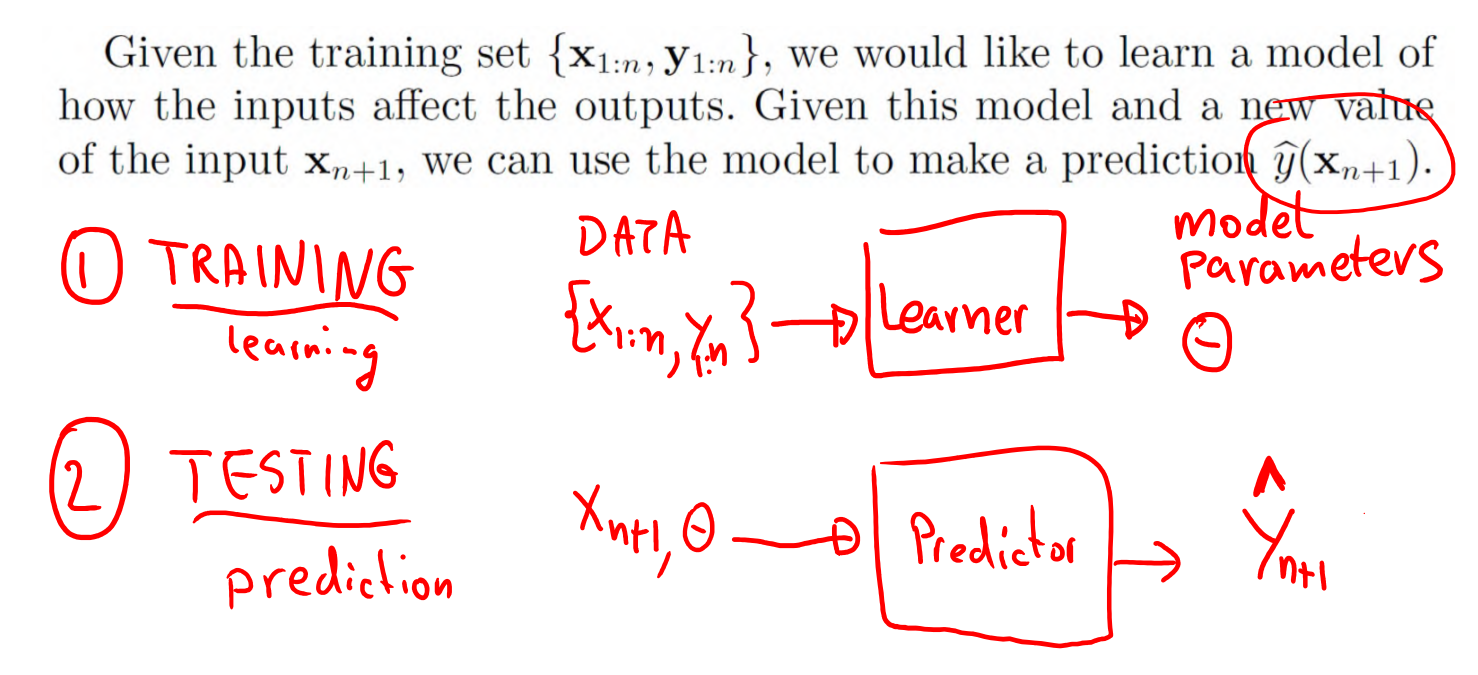
3.1 Flow-work:

Here the model is represented by parameters $\theta$, for unseen input $x_{N+1}$, to make a prediction $\hat{y}(x_{N+1})$

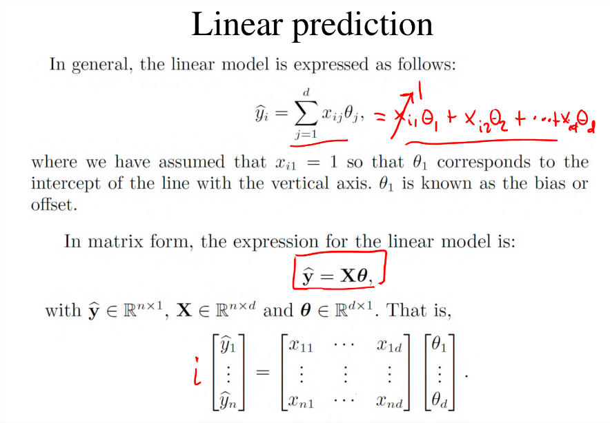
3.2 Linear Prediction

3.3 Optimization approach

Error function $J(\theta)$

$$J(\theta) \equiv (y - X\theta)^T(y - X\theta) = \sum_{i=i}^{N}{(y_i - \textbf{x}_i^T\theta)^2}$$

Finding the solution by differentiation:

Note : Matrix differentiation, $\frac{\partial{ \mathbf{A} \theta}}{\partial \theta} = \mathbf{A}^T$, and $\frac{\partial{\theta ^T \mathbf{A} \theta}}{\partial \theta} = 2\mathbf{A}^T\theta$.

We get

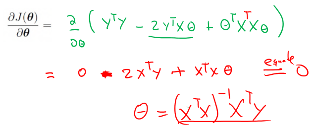
The optimal parameter $\theta ^* = \mathbf{(x^Tx)^{-1}x^Ty}$.

4. A Regression Problem: Polynomial Curve Fitting

4.1 Training data:

Given a training data set comprising N observations o x, written $\textbf{x} \equiv (x_1, ..., x_N)^T$, together with corresponding observations of the values of t, denoted $\textbf{t} \equiv (t_1, ..., t_N)^T$.

4.2 Synthetically generated data:

Method:
i.e., function value y(x) (e.g., $sin(2πx)$) + Gaussian noise.
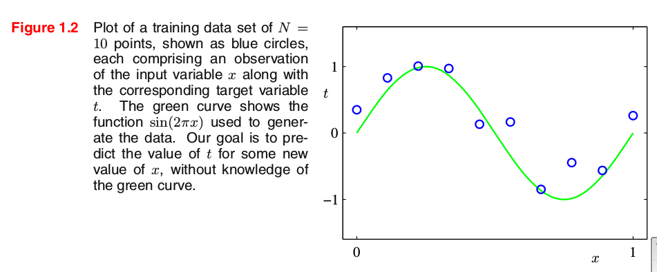
The input data set x in Figure 1.2 was generated by choosing values of $x_n$ , for $n = 1, . . . , N$ , spaced uniformly in range [0, 1], and the target data set t was obtained by first computing the corresponding values of the function sin(2πx) and then adding a small level of random noise having a Gaussian distribution to each such point in order to obtain the corresponding value $t_n$ .

Discussion:
By generating data in this way, we are capturing a property of many real data sets, namely that they possess an underlying regularity, which we wish to learn, but that individual observations are corrupted by random noise. This noise might arise from intrinsically stochastic (i.e. random) processes such as radioactive decay but more typically is due to there being sources of variability that are themselves unobserved.

4.3 Why called Linear Model?

1) polynomial function

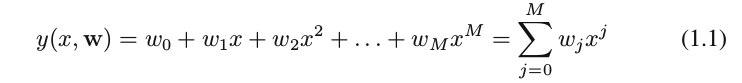
where $M$ is the order of the polynomial, and $x_j$ denotes $x$ raised to the power of $j$. The polynomial coefficients $w_ 0 , . . . , w_M$ are collectively denoted by the vector $\mathbf{w}$.

---

Question: Why called linear model or linear prediction? Why “linear”?
Answer: Note that, although the polynomial function $y(x, \theta)$ is a nonlinear function of $x$, it does be a linear function of the coefficients $\theta$. Functions, such as the polynomial, which are linear in the unknown parameters have important properties and are called linear models and will be discussed extensively in Chapters 3 and 4.

---

2) Error Function $E(\mathbf{w})$

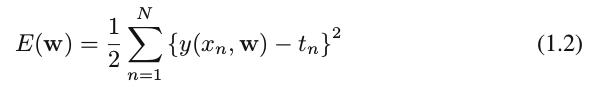
where the factor of $1/2$ is included for later convenience. We can solve the quadratic function of the coefficients $\mathbf{w}$, and find a unique optimal solution in closed form, demoted by $\mathbf{w}^*$.

4.4 Remaining Problems Related to Polynomial Curve Fitting

• Model Comparison or Model Selection: choosing the order M of the polynomial. a dilemma: large M$\uparrow$ causes over-fitting, small M$\downarrow$ gives rather poor fits to the distribution of training data.
• over-fitting: In fact, the polynomial passes exactly through each data point and E(w ) = 0. However, the fitted curve oscillates wildly and gives a very poor representation of the function $sin(2πx)$. This latter behavior is known as over-fitting.
• Model complexity: ??? # of parameters in the model.

4.5 Bayesian perspective

Least Squares (i.e., Linear Regression ) Estimate V.S. Maximum Likelihood Estimate:

We shall see that the least squares approach (i.e., linear regression) to finding the model parameters represents a specific case of maximum likelihood (discussed in Section 1.2.5), and that the over-fitting problem can be understood as a general property of maximum likelihood. By adopting a Bayesian approach, the over-fitting problem can be avoided. We shall see that there is no difficulty from a Bayesian perspective in employing models for which the number of parameters greatly exceeds the number of data points. Indeed, in a Bayesian model the effective number of parameters adapts automatically to the size of the data set.

How to formulate the likelihood for linear regression? (to be discussed in later sections.)

4.6 Regularization, Regularizer : to control over-fitting

• regularization: to involve adding a penalty term to the error function (1.2) in order to discourage the coefficients from reaching large values.

• form of regularizers: e.g., a quadratic regularizer, called ridge regression. In the context of neural networks, this approach is
  known as weight decay.

  

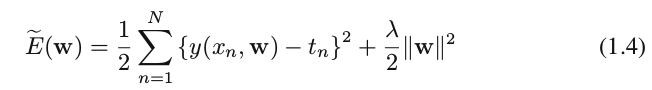
The modified error function includes two terms:
+ the first term : sum-of-squares error;
+ the second term: regularizer term, which has the desired effect of reducing the magnitude of the coefficients.

---

End of Chapter 1.1 Introduction