


在机器学习各种优化问题中,凸集、凸函数和凸优化等概念经常出现,其是各种证明的前提条件,因此认识其性质对于优化问题的理解尤为重要,本文便就凸集、凸函数和凸优化等各种性质进行阐述,文末分享一波凸优化的学习资料和视频!
一、几何体的向量表示
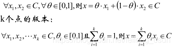
在介绍凸集等概念之前,首先介绍一下空间几何体的向量表示,下面在定义凸集概念时便用到了线段的线段表示。先通过一个例子来认识一下如何使用向量表示线段
已知二维平面上两定点A(5, 1)、B(2, 3),给出线段AB的方程表示如下:
KaTeX parse error: Expected '}', got 'EOF' at end of input: … θ∈[0, 1]
如果将点A看成向量a,点B看成向量b,则线段AB的向量表示为:
x → = θ a → + ( 1 − θ ) ∗ b → θ ∈ [ 0 , 1 ] x → = θ a → + ( 1 − θ ) ∗ b → θ ∈ [ 0 , 1 ] x = θ a + ( 1 − θ ) ∗ b θ ∈ [ 0 , 1 ] x→=θa→+(1−θ)∗b→ θ∈[0, 1] \overrightarrow{x} = \theta\overrightarrow{a} + \left( 1 - \theta \right)*\overrightarrow{b}\ \ \ \ \ \ \ \theta \in \lbrack 0,\ 1\rbrack x=θa+(1−θ)∗b θ∈[0, 1] x→=θa→+(1−θ)∗b→ θ∈[0, 1]x=θa+(1−θ)∗b θ∈[0, 1]x=θa+(1−θ)∗b θ∈[0, 1]
而直线的向量表示是:
x → = θ a → + ( 1 − θ ) ∗ b → θ ∈ R x → = θ a → + ( 1 − θ ) ∗ b → θ ∈ R x = θ a + ( 1 − θ ) ∗ b θ ∈ R x→=θa→+(1−θ)∗b→ θ∈R \overrightarrow{x} = \theta\overrightarrow{a} + \left( 1 - \theta \right)*\overrightarrow{b}\ \ \ \ \ \ \ \theta \in R x=θa+(1−θ)∗b θ∈R x→=θa→+(1−θ)∗b→ θ∈Rx=θa+(1−θ)∗b θ∈Rx=θa+(1−θ)∗b θ∈R
由此衍生推广到高维,可得以下几何体的向量表示,三角形的向量表示:
x → = θ 1 a → 1 + θ 2 a → 2 + θ 3 a → 3 θ i ∈ [ 0 , 1 ] a n d ∑ θ i = 1 x → = θ 1 a → 1 + θ 2 a → 2 + θ 3 a → 3 θ i ∈ [ 0 , 1 ] and ∑ θ i = 1 x = θ 1 a 1 + θ 2 a 2 + θ 3 a 3 θ i ∈ [ 0 , 1 ] a n d ∑ θ i = 1 x→=θ1a→1+θ2a→2+θ3a→3 θi∈[0, 1] and ∑θi=1 \overrightarrow{x} = \theta_{1}{\overrightarrow{a}}_{1} + \theta_{2}{\overrightarrow{a}}_{2} + \theta_{3}{\overrightarrow{a}}_{3}\text{\ \ \ \ \ \ }\theta_{i} \in \left\lbrack 0,\ 1 \right\rbrack\text{\ and\ }\sum_{}^{}\theta_{i} = 1 x=θ1a1+θ2a2+θ3a3 θi∈[0, 1] and ∑θi=1 x→=θ1a→1+θ2a→2+θ3a→3 θi∈[0, 1] and ∑θi=1x=θ1a1+θ2a2+θ3a3 θi∈[0, 1] and ∑θi=1x=θ1a1+θ2a2+θ3a3 θi∈[0, 1] and ∑θi=1
三维平面的向量表示:
x → = θ 1 a → 1 + θ 2 a → 2 + θ 3 a → 3 θ i ∈ R a n d ∑ θ i = 1 x → = θ 1 a → 1 + θ 2 a → 2 + θ 3 a → 3 θ i ∈ R and ∑ θ i = 1 x = θ 1 a 1 + θ 2 a 2 + θ 3 a 3 θ i ∈ R a n d ∑ θ i = 1 x→=θ1a→1+θ2a→2+θ3a→3 θi∈R and ∑θi=1 \overrightarrow{x} = \theta_{1}{\overrightarrow{a}}_{1} + \theta_{2}{\overrightarrow{a}}_{2} + \theta_{3}{\overrightarrow{a}}_{3}\text{\ \ \ \ \ \ }\theta_{i} \in R\text{\ and\ }\sum_{}^{}\theta_{i} = 1 x=θ1a1+θ2a2+θ3a3 θi∈R and ∑θi=1 x→=θ1a→1+θ2a→2+θ3a→3 θi∈R and ∑θi=1x=θ1a1+θ2a2+θ3a3 θi∈R and ∑θi=1x=θ1a1+θ2a2+θ3a3 θi∈R and ∑θi=1
超几何体的向量表示:
x → = θ 1 a → 1 + θ 2 a → 2 + … + θ k a → k θ i ∈ [ 0 , 1 ] a n d ∑ θ i = 1 x → = θ 1 a → 1 + θ 2 a → 2 + … + θ k a → k θ i ∈ [ 0 , 1 ] and ∑ θ i = 1 x = θ 1 a 1 + θ 2 a 2 + … + θ k a k θ i ∈ [ 0 , 1 ] a n d ∑ θ i = 1 x→=θ1a→1+θ2a→2+…+θka→k θi∈[0, 1] and ∑θi=1 \overrightarrow{x} = \theta_{1}{\overrightarrow{a}}_{1} + \theta_{2}{\overrightarrow{a}}_{2} + \ldots + \theta_{k}{\overrightarrow{a}}_{k}\text{\ \ \ \ \ \ }\theta_{i} \in \lbrack 0,\ 1\rbrack\text{\ and\ }\sum_{}^{}\theta_{i} = 1 x=θ1a1+θ2a2+…+θkak θi∈[0, 1] and ∑θi=1 x→=θ1a→1+θ2a→2+…+θka→k θi∈[0, 1] and ∑θi=1x=θ1a1+θ2a2+…+θkak θi∈[0, 1] and ∑θi=1x=θ1a1+θ2a2+…+θkak θi∈[0, 1] and ∑θi=1
超平面的向量表示:
x → = θ 1 a → 1 + θ 2 a → 2 + … + θ k a → k θ i ∈ R a n d ∑ θ i = 1 x → = θ 1 a → 1 + θ 2 a → 2 + … + θ k a → k θ i ∈ R and ∑ θ i = 1 x = θ 1 a 1 + θ 2 a 2 + … + θ k a k θ i ∈ R a n d ∑ θ i = 1 x→=θ1a→1+θ2a→2+…+θka→k θi∈R and ∑θi=1 \overrightarrow{x} = \theta_{1}{\overrightarrow{a}}_{1} + \theta_{2}{\overrightarrow{a}}_{2} + \ldots + \theta_{k}{\overrightarrow{a}}_{k}\text{\ \ \ \ \ \ }\theta_{i} \in R\text{\ and\ }\sum_{}^{}\theta_{i} = 1 x=θ1a1+θ2a2+…+θkak θi∈R and ∑θi=1 x→=θ1a→1+θ2a→2+…+θka→k θi∈R and ∑θi=1x=θ1a1+θ2a2+…+θkak θi∈R and ∑θi=1x=θ1a1+θ2a2+…+θkak θi∈R and ∑θi=1
二、凸集凸函数定义
1、凸集
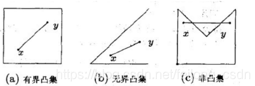
集合C内任意两点间的线段也均在集合C内,则称集合C为凸集,数学定义为:
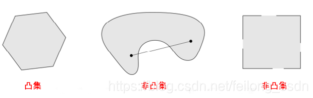
上面凸集定义中便用到了线段的向量表示,含义是如果点x1和点x2在集合C内,则线段x1x2上所有点都在集合c内,凸集的交集仍是凸集,下面展示几个凸集示例:
2、凸函数
凸函数定义为:
KaTeX parse error: Expected 'EOF', got '&' at position 9: f:C⊆ Rn−&̲gt;R1, C.x1,x2∈…
KaTeX parse error: Expected 'EOF', got '&' at position 13: f(α1x1+α2x2)&̲lt;= α1f(x1)+ α…
则成 f(x) 为定义在凸集C上的凸函数
严格凸函数定义:设 f ⊆ Rn–> R1,C是凸集,对于x1, x2∈C 都有:
KaTeX parse error: Expected 'EOF', got '&' at position 13: f(α1x1+α2x2)&̲lt; α1f(x1)+ α2…
则成 f(x) 为定义在凸集C上的严格凸函数
凸函数的等价定义:设f ⊆ Rn–> R1,C是凸集,对于x1, x2, x3∈C且x1<x2<x3,下式成立则 f(x) 为凸函数:
KaTeX parse error: Expected 'EOF', got '&' at position 19: …2)− f(x1)x2− x1&̲lt;= f(x3)− f(x…
3、凸函数定义几何解释
对于凸函数公式描述:
KaTeX parse error: Expected 'EOF', got '&' at position 13: f(α1x1+α2x2)&̲lt;= α1f(x1)+ α…
如下图所示,设A1、A2是凸函数曲线上的两个点,他们对应的横坐标x1<x2,且x∈(x1, x2),则存在 α1, α2>0且 α1+ α2=1,使得x= α1x1+ α2x2,过点x做x轴的垂线交函数于A,交直线A1A2于B点,则上式左端即为A的纵坐标,右端即为B的纵坐标:
y A = f ( α 1 x 1 + α 2 x 2 ) y A = f ( α 1 x 1 + α 2 x 2 ) y A = f ( α 1 x 1 + α 2 x 2 ) yA= f(α1x1+α2x2) y_{A} = \ f\left( \alpha_{1}x_{1} + \alpha_{2}x_{2} \right) yA= f(α1x1+α2x2) yA= f(α1x1+α2x2)yA= f(α1x1+α2x2)yA= f(α1x1+α2x2)
y B = α 1 f ( x 1 ) + α 2 f ( x 2 ) y B = α 1 f ( x 1 ) + α 2 f ( x 2 ) y B = α 1 f ( x 1 ) + α 2 f ( x 2 ) yB=α1f(x1)+ α2f(x2) y_{B} = \alpha_{1}f\left( x_{1} \right) + \ \alpha_{2}f\left( x_{2} \right) yB=α1f(x1)+ α2f(x2) yB=α1f(x1)+ α2f(x2)yB=α1f(x1)+ α2f(x2)yB=α1f(x1)+ α2f(x2)
因此,凸函数的几何含义是:函数任意两点A1和A2之间的部分位于弦A1A2的下方或曲线任一点切线上方,不严谨一个说法:割线始终位于两点间函数曲线的上方

三、凸函数各种性质及其证明
1、性质1:设 f ⊆ Rn–> R1,C是凸集,若f是凸函数,则对于∀β,证明下面水平集Dβ是凸集
KaTeX parse error: Expected '}', got '&' at position 11: Dβ={x∣f(x)&̲lt;=β, x∈C} D_{…
证明一个集合是凸集,按照凸集性质即证明凸集中任意两点构成的线段仍然在凸集内,证明见下图:

2、性质2:凸优化问题的局部极小值是全局极小值
这个性质是凸优化问题一个良好的性质,在机器学习任务中我们只需将非凸问题转化为凸优化问题,便可直接求出问题的全局极值,下面给出证明:

我们观察下面两幅图,形象感受一下为什么凸优化问题的局部最优解是全局最优解
(1) 从下图可以看出当函数不是凸函数时,当对非凸函数f(x)进行最优化时,便可能得到局部最优解,无法获得全局最优解

(2) 从下图可以看出当目标函数可行域是非凸时,则此时对函数进行优化时也可能错过全局最优解

3、性质3:设 f ⊆ Rn–> R1,C是凸集,对于x1, x2∈C
(1) f为凸函数的充要条件是:对于∀x1, x2∈C且x1≠x2都有:
KaTeX parse error: Expected 'EOF', got '&' at position 6: f(x2)&̲gt;f(x1)+ ∇f(x1…
(2) f为严格凸函数的充要条件是:对于∀x1, x2∈C且x1≠x2都有:
KaTeX parse error: Expected 'EOF', got '&' at position 6: f(x2)&̲gt;= f(x1)+ ∇f(…
证明过程如下:


性质3描述的凸函数一阶可微时具有的性质,下面给出该性质的几何解释

看上图,凸函数f(x),在函数f(x)上取一点(x, f(x))做曲线的切线,切线的斜率为k,可以看出对于凸函数f(x)来说,切线始终是凸函数f(x)的下界,我们看点A、B,B是曲线上一点,A点是切线上一点,且A、B的横坐标都为y,则B点的纵坐标始终大于A点的纵坐标,于是便可得到上述性质:
f ( y ) ≥ f ( x ) + ∇ f ( x ) T ( y − x ) f ( y ) ≥ f ( x ) + ∇ f ( x ) T ( y − x ) f ( y ) ≥ f ( x ) + ∇ f ( x ) T ( y − x ) f(y)≥f(x)+ ∇f(x)T(y−x) f\left( y \right) \geq f\left( x \right) + \ \nabla{f\left( x \right)}^{T}(y - x) f(y)≥f(x)+ ∇f(x)T(y−x) f(y)≥f(x)+ ∇f(x)T(y−x)f(y)≥f(x)+ ∇f(x)T(y−x)f(y)≥f(x)+ ∇f(x)T(y−x)
当y不断逼近x时,则上式等号成立
4、性质4:凸函数其Hessian矩阵半正定
性质4描述的凸函数二阶可微时满足的性质,即凸函数Hessian矩阵半正定,此性质可通过泰勒公式进行,在给出该性质证明之前,Hessian矩阵和泰勒公式定义
Hessian矩阵是一个多元函数的二阶偏导数构成的方阵,一个多元函数Hessian矩阵定义如下:

泰勒公式是用若干项连加来表示一个函数,这些相加的项由函数在某一点的导数求得,下面给出一个函数f(x)在x=a点的泰勒展开式:

上述性质凸函数其Hessian矩阵半正定的证明如下:

5、性质5:若 x ⊆ Rn,y⊆ Rn,Q为半正定对称阵,证明f(x) = XTQX为凸函数

6、性质6:凸函数f(x),其中Q1+Q2+…+Qn=1,0<= Qi<=1,证明下面不等式:
KaTeX parse error: Expected 'EOF', got '&' at position 21: …1+Q2x2+…+Qnxn+)&̲lt;= Q1f(x1)+Q2…

7、Jessen不等式,f(x)为凸函数,其中E(x)是x的期望,证明:
KaTeX parse error: Expected 'EOF', got '&' at position 8: f(E(x))&̲lt;=E(f(x)) f\l…

四、凸优化定义
1、凸优化问题定义
一个凸优化问题可描述为:
f ( x ) s . t . x ∈ C f ( x ) s . t . x ∈ C f ( x ) s . t . x ∈ C f(x) s.t. x∈C \operatorname{}{f\left( x \right)}\text{\ \ \ \ \ }s.t.\ \ x \in C f(x) s.t. x∈C f(x) s.t. x∈Cf(x) s.t. x∈Cf(x) s.t. x∈C
KaTeX parse error: Expected 'EOF', got '&' at position 12: s.t. gi(x)&̲lt;=0 hi(x) =0…
通过以下凸优化性质便可理解何为凸优化问题:
(1) 目的是求解目标函数的最小值;
(2) 目标函数f(x)和不等式约束函数g(x)都是凸函数,定义域是凸集;
(3) 若存在等式约束函数,则等式约束函数h(x)为仿射函数;仿射函数指的是最高次数为1的多项式函数,一般形式为f(x)= Ax + b,A是m*k矩阵,x是一个k向量,b是一个m向量
(4) 凸优化问题有一个良好的性质即:局部最优解便是全局最优解
2、常见凸优化问题
(1) 线性规划LinearProgramming(LP)
如果目标函数和不等式约束函数都是仿射函数,则凸优化问题称为线性规划,数学表示为:
c T x + d c T x + d c T x + d cTx+d \operatorname{}{c^{T}x} + d cTx+d cTx+dcTx+dcTx+d
s . t . G x ≼ h A x = b s . t . G x ≼ h A x = b s . t . G x ≼ h A x = b s.t. Gx ≼h Ax=b s.t.\ \ Gx\ \preccurlyeq h\ \ \ Ax = b s.t. Gx ≼h Ax=b s.t. Gx ≼h Ax=bs.t. Gx ≼h Ax=bs.t. Gx ≼h Ax=b
(2) 二次规划QuadraticProgramming(QP)
如果目标函数是凸二次函数,而不等式约束仍是仿射函数,则凸优化问题称为二次规划,数学表示为:
12 x T P x + c T x + d 1 2 x T P x + c T x + d 21 x T P x + c T x + d 12xTPx+cTx+d \operatorname{}\frac{1}{2}x^{T}Px + c^{T}x + d 21xTPx+cTx+d 12xTPx+cTx+d21xTPx+cTx+d21xTPx+cTx+d
s . t . G x ≺ = h A x = b s . t . G x ≺ = h A x = b s . t . G x ≺ = h A x = b s.t. Gx ≺=h Ax=b s.t.\ \ Gx\ \prec = h\ \ \ Ax = b s.t. Gx ≺=h Ax=b s.t. Gx ≺=h Ax=bs.t. Gx ≺=h Ax=bs.t. Gx ≺=h Ax=b
(3) 二次约束的二次规划Quadratically Constrained Quadratic Programming(QCQP)
如果目标函数和不等书约束均为凸二次函数,则凸优化问题称为二次约束的二次规划,数学表示为:
12 x T P x + c T x + d 1 2 x T P x + c T x + d 21 x T P x + c T x + d 12xTPx+cTx+d \operatorname{}\frac{1}{2}x^{T}Px + c^{T}x + d 21xTPx+cTx+d 12xTPx+cTx+d21xTPx+cTx+d21xTPx+cTx+d
s . t . 12 x T Q i x + r i T x + s i ≤ 0 i = 1 , 2 , … , m A x = b s.t. 1 2 x T Q i x + r i T x + s i ≤ 0 i = 1 , 2 , … , m A x = b s . t . 21 x T Q i x + r i T x + s i ≤ 0 i = 1 , 2 , … , m A x = b s.t. 12xTQix+riTx+si≤0 i=1,2,…,m Ax=b \text{s.t.\ \ }\frac{1}{2}x^{T}Q_{i}x + r_{i}^{T}x + s_{i} \leq 0\ \ \ \ i = 1,2,\ldots,m\ \ Ax = b s.t. 21xTQix+riTx+si≤0 i=1,2,…,m Ax=b s.t. 12xTQix+riTx+si≤0 i=1,2,…,m Ax=bs.t. 21xTQix+riTx+si≤0 i=1,2,…,m Ax=bs.t. 21xTQix+riTx+si≤0 i=1,2,…,m Ax=b
(4) 半正定规划Semidefinite Programming(SDP)
半正定规划较前面的复杂,在机器学习中也经常用到,下面给出数学描述:
t r ( C X ) t r ( C X ) t r ( C X ) tr(CX) \operatorname{}{tr(CX)} tr(CX) tr(CX)tr(CX)tr(CX)
s . t . t r ( A i x ) = b i i = 1 , 2 , … , p X ≽ 0 s.t. tr ( A i x ) = b i i = 1 , 2 , … , p X ≽ 0 s . t . t r ( A i x ) = b i i = 1 , 2 , … , p X ≽ 0 s.t. tr(Aix)=bi i=1,2,…,p X≽0 \text{s.t.\ \ tr}\left( A_{i}x \right) = b_{i}\ \ \ \ i = 1,2,\ldots,p\ \ \ X \succcurlyeq 0 s.t. tr(Aix)=bi i=1,2,…,p X≽0 s.t. tr(Aix)=bi i=1,2,…,p X≽0s.t. tr(Aix)=bi i=1,2,…,p X≽0s.t. tr(Aix)=bi i=1,2,…,p X≽0
其中符号tr(A)表示矩阵A的迹,矩阵A的迹是指A的对角线上各个元素的总和
五、浅谈凸优化问题为何如此重要
1、凸优化具有良好性质,如局部最优解是全局最优解,且凸优化问题是多项式时间可解问题,如:线性规划问题;
2、很多非凸优化或NP-Hard问题可以转化成凸优化问题,方法:对偶、松弛(扩大可行域,去掉部分约束条件),在SVM算法中,为了对目标函数进行优化,便使用了拉格朗日乘子法、对偶问题、引入松弛因子等
凸优化资料:百度云盘链接,密码:ei8e
</div>
<link href="https://csdnimg.cn/release/phoenix/mdeditor/markdown_views-b6c3c6d139.css" rel="stylesheet">
<div class="more-toolbox">
<div class="left-toolbox">
<ul class="toolbox-list">
<li class="tool-item tool-active is-like "><a href="javascript:;"><svg class="icon" aria-hidden="true">
<use xlink:href="#csdnc-thumbsup"></use>
</svg><span class="name">点赞</span>
<span class="count">17</span>
</a></li>
<li class="tool-item tool-active is-collection "><a href="javascript:;" data-report-click="{"mod":"popu_824"}"><svg class="icon" aria-hidden="true">
<use xlink:href="#icon-csdnc-Collection-G"></use>
</svg><span class="name">收藏</span></a></li>
<li class="tool-item tool-active is-share"><a href="javascript:;"><svg class="icon" aria-hidden="true">
<use xlink:href="#icon-csdnc-fenxiang"></use>
</svg>分享</a></li>
<!--打赏开始-->
<!--打赏结束-->
<li class="tool-item tool-more">
<a>
<svg t="1575545411852" class="icon" viewBox="0 0 1024 1024" version="1.1" xmlns="http://www.w3.org/2000/svg" p-id="5717" xmlns:xlink="http://www.w3.org/1999/xlink" width="200" height="200"><defs><style type="text/css"></style></defs><path d="M179.176 499.222m-113.245 0a113.245 113.245 0 1 0 226.49 0 113.245 113.245 0 1 0-226.49 0Z" p-id="5718"></path><path d="M509.684 499.222m-113.245 0a113.245 113.245 0 1 0 226.49 0 113.245 113.245 0 1 0-226.49 0Z" p-id="5719"></path><path d="M846.175 499.222m-113.245 0a113.245 113.245 0 1 0 226.49 0 113.245 113.245 0 1 0-226.49 0Z" p-id="5720"></path></svg>
</a>
<ul class="more-box">
<li class="item"><a class="article-report">文章举报</a></li>
</ul>
</li>
</ul>
</div>
</div>
<div class="person-messagebox">
<div class="left-message"><a href="https://blog.csdn.net/feilong_csdn">
<img src="https://profile.csdnimg.cn/8/E/9/3_feilong_csdn" class="avatar_pic" username="feilong_csdn">
<img src="https://g.csdnimg.cn/static/user-reg-year/1x/4.png" class="user-years">
</a></div>
<div class="middle-message">
<div class="title"><span class="tit"><a href="https://blog.csdn.net/feilong_csdn" data-report-click="{"mod":"popu_379"}" target="_blank">feilong_csdn</a></span>
</div>
<div class="text"><span>发布了52 篇原创文章</span> · <span>获赞 313</span> · <span>访问量 36万+</span></div>
</div>
<div class="right-message">
<a href="https://im.csdn.net/im/main.html?userName=feilong_csdn" target="_blank" class="btn btn-sm btn-red-hollow bt-button personal-letter">私信
</a>
<a class="btn btn-sm bt-button personal-watch" data-report-click="{"mod":"popu_379"}">关注</a>
</div>
</div>
</div>


 1万+
1万+


 被折叠的 条评论
为什么被折叠?
被折叠的 条评论
为什么被折叠?
 到【灌水乐园】发言


