


一、 ROC曲线
1. 混淆矩阵
针对二分类问题,将实例分成正类(postive)或者负类(negative)。但是实际中分类时,会出现四种情况.
(1)若一个实例是正类并且被预测为正类,即为真正类(True Postive TP)
(2)若一个实例是正类,但是被预测成为负类,即为假负类(False Negative FN)
(3)若一个实例是负类,但是被预测成为正类,即为假正类(False Postive FP)
(4)若一个实例是负类,但是被预测成为负类,即为真负类(True Negative TN)
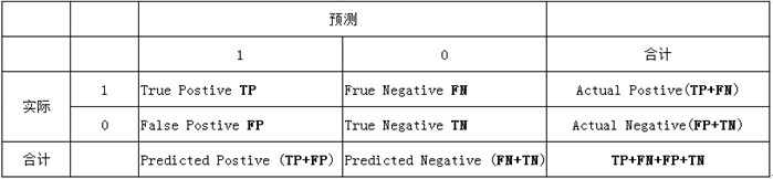
分类模型的性能根据模型正确和错误预测的检验记录计数进行评估,这些计数存放在称作混淆矩阵(confusion matrix)的表格中
由上表可得出横,纵轴的计算公式:
(1)真正类率(True Postive Rate)TPR: TP/(TP+FN),代表分类器预测的正类中实际正实例占所有正实例的比例。Sensitivity ——- 纵坐标
(2)负正类率(False Postive Rate)FPR: FP/(FP+TN),代表分类器预测的正类中实际负实例占所有负实例的比例。1-Specificity —— 横坐标
(3)真负类率(True Negative Rate)TNR: TN/(FP+TN),代表分类器预测的负类中实际负实例占所有负实例的比例,TNR=1-FPR。Specificity
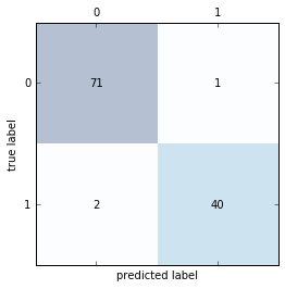
2. Python绘制混淆矩阵
# scikit-learn 计算混淆矩阵
from sklearn.metrics import confusion_matrix
Model.fit(X_train,y_train)
y_pred = Model.predict(X_test)   # Model根据选择的不同模型,写法不同
confmat = confusion_matrix(y_true=y_test, y_pred=y_pred)
print(confmat)
# [[71 1]
# [ 2 40]]
# 绘制混淆矩阵
fig,ax= plt.subplots()
ax.matshow(confmat, cmap=plt.cm.Blues, alpha=0.3)
for i in range(confmat.shape[0]):
    for j in range(confmat.shape[1]):
        ax.text(x=j, y=i, s=confmat[i,j],va='center', ha='center')
plt.xlabel('predicted label')
plt.ylabel('true label')
plt.show()
3.ROC曲线
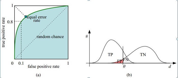
接收者操作特征(receiver operating characteristic),roc曲线上每个点反映着对同一信号刺激的感受性
横轴:负正类率(false positive rate,FPR)特异度 Specificity
代表分类器预测的正类中实际负实例占所有负实例的比例。1-Specificity
纵轴:真正类率(true positive rate,TPR)灵敏度 Sensitivity(正类覆盖率)
代表分类器预测的正类中实际正实例占所有正实例的比例。Sensitivity
横轴FPR:1-TNR,1-Specificity,FPR越大,预测正类中实际负类越多。
纵轴TPR:Sensitivity(正类覆盖率),TPR越大,预测正类中实际正类越多。
理想目标:TPR=1,FPR=0,即图中(0,1)点,故ROC曲线越靠拢(0,1)点,越偏离45度对角线越好,Sensitivity、Specificity越大效果越好。
4.Python 绘制ROC曲线
from sklearn.metrics import roc_curve, auc
from scipy import interp  # interp 线性插值
X_train2 = X_train[:, [4,14]]
cv = StratifiedKFold(y_train, n_folds=3, random_state=1)
fig = plt.figure()
mean_tpr=0.0
mean_fpr=np.linspace(0,1,100)
all_tpr = []
# plot 每个fold的ROC曲线,这里fold的数量为3,被StratifiedKFold指定
for i, (train,test) in enumerate(cv):
    #返回预测的每个类别(这里为0或1)的概率  probas[:,0] – 预测为0的概率,probas[:,1]—预测为1的概率
    probas = pipe_lr.fit(X_train2[train],y_train[train]).predict_proba(X_train2[test])
    fpr,tpr,thresholds = roc_curve(y_train[test],probas[:,1],pos_label=1)
    mean_tpr += interp(mean_fpr, fpr,tpr)
    mean_tpr[0]=0.0
    roc_auc=auc(fpr,tpr)
    plt.plot(fpr,tpr,linewidth=1,label='ROC fold %d (area = %0.2f)' % (i+1, roc_auc))
# plot random guessing line
plt.plot([0,1],[0,1],linestyle='--',color=(0.6,0.6,0.6),label='random guessing')
mean_tpr /= len(cv)
mean_tpr[-1] = 1.0
mean_auc = auc(mean_fpr, mean_tpr)
plt.plot(mean_fpr, mean_tpr, 'k--', label='mean ROC (area = %0.2f)' % mean_auc, lw=2)


# plot perfect performance line
plt.plot([0, 0, 1], [0, 1, 1], lw=2, linestyle=':', color='black', label='perfect performance')
# 设置x,y坐标范围
plt.xlim([-0.05,1.05])
plt.ylim([-0.05,1.05])
plt.xlabel('false positive rate')
plt.ylabel('true positive rate')
plt.title('Receiver Operator Charateristic')
plt.legend(loc='lower right')
plt.show()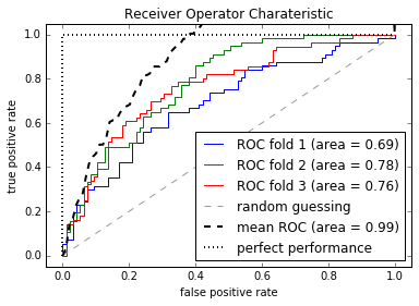


 8632
8632

 被折叠的 条评论
为什么被折叠?
被折叠的 条评论
为什么被折叠?
 到【灌水乐园】发言


