Graph Coarsening And multi-source BFS

Coarsening

[何慧, 胡铭曾, 张宏莉, 裴晓峰, & 杨志. (2005). 网络拓扑图多级分割塌缩阶段算法改进. 华中科技大学学报:自然科学版, 33(S1), 82-85.]
图塌缩阶段是将图中联系较强部分粘合起来 作为一个整体, 并暂时从图中隐藏掉.这样经过多 次塌缩后 ,使图变小 .例如一个复杂的数千条边的 图会经塌缩阶段变成只有数十条甚至更少边数的 图,这样通过对简单图进行初始划分容易得到较 好的划分结果.初始划分后,再按照塌缩步骤逆序 恢复并优化,最终还原成原图 ,得到一条多级划分 的分割线.此算法目前有多级二分法和多级 K 分 法两种.
目前塌缩算法时间复杂度大多是 O( E ), 并且对于图塌缩算法去寻找图的最大塌缩匹配. 这里提出一个与塌缩边相对应的塌缩算法———顶 点塌缩算法.
2.1 关键顶点塌缩(KV)算法
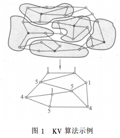
塌缩算法主要目的是尽可能减少初始划分难 度,尽可能减少图分割边的数目.而对于分割边来 说,如果权重比较大的边都被塌缩掉的话,对剩余 图进行初始划分得到的结果, 就会是分割边权重 较小的划分方法.如图 1 所示 ,考虑从节点出发, 塌缩算法针对的是拥有重权边的顶点 , 那么塌缩 掉的部分将会有比较高的权重, 并且尽可能塌缩 掉大度顶点,以减少分割边增大的概率 .

以 a(v)表示顶点 v 所有关联边的边权和, 对于 a(v)较大的点 , 可以认为与其关联的边都 是拥有比较关键作用的, 这样边权才会较大 ,因此 将这些顶点称之为关键顶点(Key Vertex), 如果 将这些顶点和与之相连的边都塌缩掉 , 那么塌缩 的将是图中边权较重部分 . 下面给出对于有权图的 KV 算法描述:
a.统计计算图顶点的 a (v),依序保存在二 叉树 S 中;
b .依大小顺序 ,访问 a(v)最大顶点 v_i ,从图的邻接表 B 中查询与 v_i 相邻顶点 , 与 v_i 一起塌缩成一个顶点v′_i,从二叉树 中删除这些顶点 ;
c.生成新图的邻接表 B′, 原本与 v_i 相邻顶 点关联的边都附着到 v′_i 上去;
d .修改塌缩后顶点权值 ,其值等于所有塌缩 顶点权值和;
e.在新邻接表 B′中查询新顶点 v′_i 的相邻顶 点,把这些顶点从二叉树 S 中删除;
f.如果二叉树中还有顶点,则返回 b ,否则算 法结束.
本算法时间复杂度是 O( V log( V )),但 如果不考虑第一步对二叉树按序插入 , 本算法时 间复杂度是 O( E ).虽然算法单轮时间复杂度 是 O( V log( V )), 但由于是范围塌缩 ,每轮 塌缩程度要大于边塌缩算法, 所以实际执行时间 相对 O( E )来说也是可以接受的 .
2.2 顶点团塌缩(Vertex Clique)算法
出于对上述算法时间复杂度考虑 ,尝试将关 键节点塌缩也按照上文描述采用随机访问顶点方 式来达到 O( E )时间复杂度.在不对顶点按照 其度大小或者 a(v)大小排序的情况下, 改进算 法思路仍然只能回归到在选择随机访问到的顶点 关联边中选择一条.
依照关键顶点塌缩算法, 期望选中的边连接 的是两个计算负载较重的边, 同时这条边本身也 是负载较重的边 .在给出算法之前 ,先给出衡量选 择边的标准.

Multi-source BFS

[ The More the Merrier: Efficient Multi-Source Graph Traversal ]

• Text Note, page 1
  算法的大概意思: 在将遍历的当前顶点的邻居压如 NearestQueue <v′, bfs_operator′>时, 加入即将要对它进行遍历的 bfs_operator, 下次遍历的时候, 仅仅选择一个 operator 进行操作.

• Anchored Note, page 1
  I

• Highlight, page 1
  (i) shares common computation across concurrent BFSs; (ii) greatly reduces the number of random memory accesses during BFS; and (iii) does not in- cur synchronization costs.

• Highlight, page 1
  ever-growing 日益增长

• Highlight, page 1
  To better comprehend and assess the relationships between entities in this data, and to uncover patterns and new insights, graph analytics has become essential.

• Highlight, page 1
  Often, the best one can do with existing approaches in order to reduce the overall runtime is to execute multiple single-threaded BFSs in par- allel, instead of running parallel BFSs sequentially, because the former avoids synchronization and data transfer costs,

• Highlight, page 2
  MS-BFS takes an orthogonal approach from previ- ous work: instead of parallelizing a single BFS, we focus on processing a large number of BFSs concurrently in a sin- gle core, while still allowing to scale up to multiple cores. This approach allows us to share the computation between different BFSs without paying the synchronization cost.

• Highlight, page 3
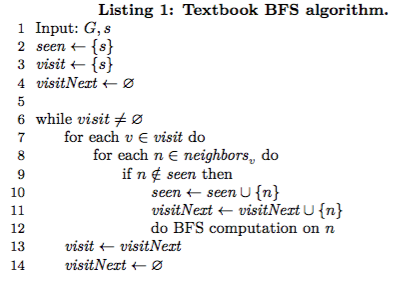
  Notably, Beamer et al. [8] propose a bottom-up ap- proach to avoid many failed checks to seen as mentioned before. I

• Underline, page 4
  B, S

• Highlight, page 4
  we propose an approach to concurrently run multiple BFSs and to share the exploration of vertices across these BFSs by leveraging the properties of small-world networks.

• Highlight, page 4
  presented in the previous sec- tion, are orthogonal to our goal: they optimize the runtime execution of a single BFS, while we want to optimize the run- time execution for multiple BFSs.

• Highlight, page 4
  Figure 1 depicts, for every BFS level, the percentage of vertex explorations that can be shared by at least 2, 50, 100, and 250 BFSs out of 512 concurrent BFSs as indicated by the bar height and color. Note that the exploration of more than 70% of the vertices in levels 3 and 4 can be shared among at least 100 BFSs, and in level

• Highlight, page 5
  4, more than 60% of them can be shared by at least 250 BFSs.

• Highlight, page 5
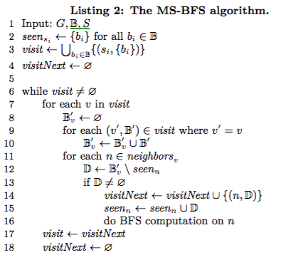
  B = {b1,...,bω}, where each bi represents a BFS, and ω is the total number of BFSs to be executed. Another input is the set S = {s1,...,sω} that contains the source vertex si for each BFS bi.

• Highlight, page 5
  Instead of having a single set seen of discovered vertices, each vertex v has its own set seenv ⊆ B of BFSs that have already discovered it; furthermore, the sets visit and visitNext comprise tuples (v′, B′), where the set B′ ⊆ B contains the BFSs that must explore v′.

• Highlight, page 5
  each vertex v has its own set seenv ⊆ B of BFSs that have already discovered it; furthermore, the sets visit and visitNext comprise tuples (v′, B′), where the set B′ ⊆ B contains the BFSs that must explore v′.

• Highlight, page 5
  includes in

• Highlight, page 5
  mergesallBFSsetsfromvisitthatrefertovintoasetB′v

• Highlight, page 5
  Thus, B′v contains all BFSs that will explore v in the current level, and v can then be explored only once for all of them.

• Highlight, page 5
  visitNext is used as the visit set for the next BFS level

转载于:https://my.oschina.net/u/178169/blog/675689