来自工作表单元格的Excel按钮文本

If you have buttons or shapes on an Excel  worksheet, you can get their caption text from a worksheet cell, so the text changes, based on a formula. See how to add the button, create its text, then link the button to cell text instead.

如果您在Excel工作表上有按钮或形状，则可以从工作表单元格获取其标题文本，因此该文本会根据公式进行更改。 了解如何添加按钮，创建其文本，然后将按钮链接到单元格文本。

添加工作表按钮 (Add a Worksheet Button)

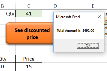
In this example, the workbook has a macro to show the total amount of an order. There's a button on the worksheet, and you click that to run the macro.

在此的示例工作簿具有一个宏，以显示订单的总额。 工作表上有一个按钮，然后单击它以运行宏。

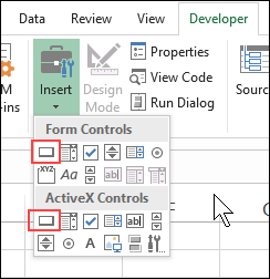
If you want to add a button, there are commands on the Developer tab, in the Insert menu on the Controls group.

如果要添加按钮，则在“控件”组的“插入”菜单中的“开发人员”选项卡上有命令。

The button in the Form Controls section is easier to use than the ActiveX controls button, and cause fewer problems, from my experience.

根据我的经验，“表单控件”部分中的按钮比ActiveX控件按钮更易于使用，并且所引起的问题更少。

The Form Controls button has an "Assign Macro" command that appears automatically, after you create it. Just choose a macro from the list, and the button is ready to use.

创建窗体控件按钮后，它会自动显示“分配宏”命令。 只需从列表中选择一个宏，该按钮即可使用。

鸽友按钮 (Fancier Buttons)

Those Developer tab buttons are okay (if you like grey), but I like to use an Excel shape instead. Shapes give you more formatting options, so you can make your button stand out on the worksheet.

这些“开发人员”选项卡按钮可以(如果您喜欢灰色)，但是我喜欢使用Excel形状。 形状为您提供了更多格式设置选项，因此您可以使按钮在工作表上突出显示。

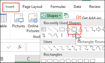
In the Insert tab of the Excel Ribbon, click Shapes, then choose one of the shapes, and click on the worksheet, where you want to add it.

在Excel功能区的“插入”选项卡中，单击“形状”，然后选择一种形状，然后在要添加形状的工作表上单击。

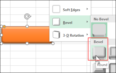
With the shape selected, you can change its height and width, other formatting options, like the fill colour and outline colour. I like to change the Shape Effects too, and give it a round Bevel, so it looks more "button=y".

选择形状后，您可以更改其高度和宽度以及其他格式设置选项，例如填充色和轮廓色。 我也喜欢更改形状效果，并给它一个圆形的斜角，所以看起来更像“ button = y”。

Then, to make the shape run a macro, right-click on the shape, and assign a macro to run when you click it.

然后，要使形状运行宏，请右键单击该形状，然后分配一个要在单击时运行的宏。

向按钮添加文本 (Add Text to the Button)

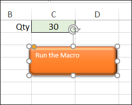
To add a caption to a shape "button", just select it, and start typing.

要将标题添加到形状“按钮”，只需选择它，然后开始输入即可。

For this button, I typed "Run the Macro"

对于此按钮，我键入了“运行宏”

格式化按钮文字 (Format the Button Text)

After you add the text, with the button still selected, use the Formatting commands on the Excel Ribbon to make the text look better.

添加文本后，仍然选择按钮，请使用Excel功能区上的“格式设置”命令使文本看起来更好。

I usually centre the text vertically and horizontally, and choose a bigger font size. Change the font colour too, if necessary, to contrast with the shape's fill colour.

我通常将文本垂直和水平居中，并选择更大的字体。 如果需要，也可以更改字体颜色，以与形状的填充色形成对比。

更改按钮文字 (Change the Button Text)

Instead of using static button text though, sometimes it's nice to have a caption that changes, based on the situation on the worksheet.

但是，代替使用静态按钮文本，有时根据工作表的情况更改标题是很好的选择。

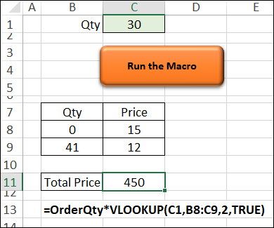
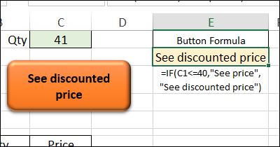
In this example, a quantity is entered in cell C1, and customers get a discount if the quantity is greater than 40.

在此示例中，在单元格C1中输入了数量，如果数量大于40，则客户将获得折扣。

The formula in the cell C11, named TotalPrice, calculates the total price of the order.

单元格C11中的公式名为TotalPrice，用于计算订单的总价。

=OrderQty * VLOOKUP(C1,B8:C9,2,TRUE)

= OrderQty * VLOOKUP(C1，B8：C9,2，TRUE)

按钮文字的公式 (Formula for Button Text)

In cell E2, I've added another formula, to check the quantity, and show text based on that amount.

在E2单元格中，我添加了另一个公式来检查数量，并根据该数量显示文本。

=IF(C1<=40,"See price", "See discounted price")

= IF(C1 <= 40，“查看价格”，“查看折扣价”)

If the quantity is 40 or less, cell E2 will show "See price". If the quantity is over 40, the result in cell E2 will mention the discount – "See discounted price"

如果数量为40个或更少，则单元格E2将显示“查看价格”。 如果数量超过40，则单元格E2中的结果将提及折扣–“查看折扣价”

将按钮文本链接到单元格 (Link Button Text to a Cell)

Instead of showing the static text, "Run the Macro", on the button, here's how to use the dynamic text from cell E2:

这里没有显示静态文本，而是在按钮上显示“运行宏”，而是如何使用单元格E2中的动态文本：

• Click on the button to select it
  点击按钮选择它

• Click in the Formula Bar, and type an equal sign:  =

  在编辑栏中单击，然后键入一个等号： =

• Click on cell E2, which has the text for the button, and press Enter
  单击单元格E2，其中包含按钮的文本，然后按Enter

NOTE: You might have to reapply some of the formatting after you link the button to the cell.

注意 ：将按钮链接到单元格后，您可能必须重新应用某些格式。

Now, it the quantity is changed, the button will show the applicable text in its caption.

现在，更改数量后，按钮将在标题中显示适用的文本。

查看步骤 (See the Steps)

This animated gif gives you a quick look at the steps.

这个动画的gif使您可以快速了解这些步骤。

切换语言 (Switch Languages)

For another example of linking shape text to worksheet cells, see the cereal box text in my "Switch Languages" blog post.

有关将形状文本链接到工作表单元格的另一个示例，请参阅我的“切换语言”博客文章中的谷物框文本 。

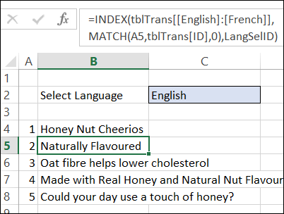
First, you select a language from a drop down list.

首先，您从下拉列表中选择一种语言。

That changes the text in the worksheet cells, because INDEX and MATCH formulas find the translations in a lookup table.

这会更改工作表单元格中的文本，因为INDEX和MATCH公式会在查找表中找到翻译。

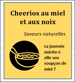
There is an orange rectangle on the worksheet, with text boxes sitting on top of it. Those text boxes are linked to the worksheet cells.

工作表上有一个橙色矩形，文本框位于其上方。 这些文本框链接到工作表单元格。

For example, the text box at the top is linked to cell B4, which shows "Honey Nut Cheerios", when English is selected.

例如，当选择英语时，顶部的文本框链接到单元格B4，该单元格显示“ Honey Nut Cheerios”。

When the selected language is French, the linked text boxes show the French text from the worksheet cells.

当所选语言为法语时，链接的文本框将显示工作表单元格中的法语文本。

翻译自: https://contexturesblog.com/archives/2019/02/28/excel-button-text-from-worksheet-cell/