excel透视表无添加字段_添加或移动数据透视表字段的快速技巧

excel透视表无添加字段

We're still recovering from Tuesday's Spreadsheet Day celebrations, so we'll keep it simple today. Here's a quick trick to add or move pivot table fields, just by typing. Watch the really short video, and there are written instructions below, if you prefer those.

我们仍在从星期二的电子表格日庆祝活动中恢复过来，因此我们今天将其简化。 这是一个仅需键入即可添加或移动数据透视表字段的快速技巧。 观看非常短的视频，如果您愿意的话，下面有书面说明。

观看视频 (Watch the Video)

Here is the short video that shows the quick trick to add or move pivot table fields, just by typing.

这是一段简短的视频，展示了只需键入即可添加或移动数据透视表字段的快速技巧。

Just make sure that you type the field name correctly! If you make a typo, you'll change the label for the existing pivot field, instead of adding the new pivot field.

只要确保您正确输入字段名称即可！ 如果输入错误，将更改现有枢轴字段的标签，而不是添加新的枢轴字段。

演示地址

添加或移动数据透视表字段 (Add or Move Pivot Table Fields)

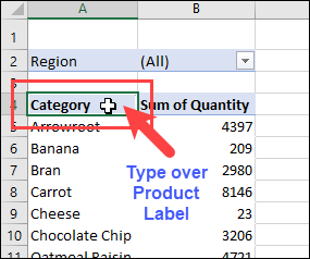
If a pivot field is not in the layout on the worksheet, you can type its name over an existing label, to add it to the layout.

如果枢轴字段不在工作表的布局中，则可以在现有标签上键入其名称，以将其添加到布局中。

Here are the steps to add or move pivot table fields on the worksheet:

以下是在工作表上添加或移动数据透视表字段的步骤：

• First, change the pivot table to Outline layout or Tabular layout. This trick will not work in Compact layout.
  首先，将数据透视表更改为“大纲”布局或“表格”布局。 此技巧不适用于紧凑型布局。
• Next, click on a cell that contains a pivot field name – a cell where you want a different field to appear
  接下来，单击包含枢轴字段名称的单元格–您要在其中显示其他字段的单元格
• Type the name of the pivot field that you want to add or move to that location
  键入要添加或移至该位置的数据透视字段的名称
• Press Enter,  to complete the pivot table  layout change.
  按Enter键以完成数据透视表布局更改。

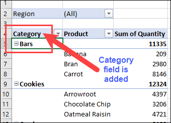
The pivot table layout changes, putting the field that you typed into the active cell. The existing fields shift down, and the added field takes its new position.

数据透视表布局发生变化，将您键入的字段放入活动单元格。 现有字段向下移动，而添加的字段占据其新位置。

移动标签的更多提示 (More Tips for Moving Labels)

The video above shows how to move pivot fields, and you can use a similar technique to move the pivot items for any pivot field.

上面的视频显示了如何移动枢轴字段，并且您可以使用类似的技术来移动任何枢轴字段的枢轴项。

The next video shows how to move the pivot items, and there are written instructions on the Move Pivot Table Labels page.

下一个视频显示了如何移动数据透视表项，并且在“移动数据透视表标签”页面上有书面说明。

演示地址

获取样本文件 (Get the Sample File)

Instead of building your own file for testing, download the Move Pivot Labels sample file from my Contextures website. The zipped file is in xlsx format, and does not contain any macros.

可以从我的Contextures网站下载“移动枢轴标签”样本文件 ，而不是构建自己的文件进行测试。 压缩文件为xlsx格式，不包含任何宏。

翻译自: https://contexturesblog.com/archives/2017/10/19/quick-trick-to-add-or-move-pivot-table-fields/

excel透视表无添加字段