如何在Excel中比较两个单元格

Aside from staring at them closely, how can you compare two cells in Excel? Here are a few functions and formulas that check the contents of two cells, to see if they are the same. We'll start with a simple check, then move up the formula ladder, for more complex comparisons.

除了盯着它们看，您如何在Excel中比较两个单元格？ 以下是一些函数和公式，用于检查两个单元格的内容，以查看它们是否相同。 我们将从简单的检查开始，然后向上移动公式阶梯，以进行更复杂的比较。

比较两个单元格的简便方法 (Easy Way to Compare Two Cells)

The quickest way to compare two cells is with a formula that uses the equal sign.

比较两个单元格的最快方法是使用使用等号的公式。

• =A2=B2

  = A2 = B2

If the cell contents are the same, the result is TRUE. (Upper and lower case versions of the same letter are treated as equal).

如果单元格内容相同，则结果为TRUE。 (同一字母的大写和小写版本被视为相等)。

忽略多余的空间 (Ignore Extra Spaces)

If you just want to compare two cells, but aren't concerned about leading spaces, trailing spaces, or extra spaces, use the TRIM function to remove them, for one or both of the cells.

如果您只想比较两个单元格，而又不关心前导空格，尾随空格或多余的空格，请对一个或两个单元格使用TRIM函数删除它们。

• =TRIM(A2)=TRIM(B2)

  = TRIM(A2)= TRIM(B2)

That can help if you're trying to match text strings to the values in an imported list, such as this VLOOKUP example.

如果您尝试将文本字符串与导入列表中的值进行匹配(例如此VLOOKUP示例) ，则可能会有所帮助。

精确比较两个单元格 (Compare Two Cells Exactly)

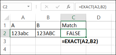
If you need to compare two cells for contents and upper/lower case, use the EXACT function. As its name indicate, that function can check for an exact match between text strings, including upper and lower case. It doesn't test the formatting though, so it won't detect if one cell has some or all of the characters in bold, and the other cell doesn't.

如果需要比较两个单元格的内容和大写/小写，请使用EXACT函数。 顾名思义，该函数可以检查文本字符串之间的精确匹配，包括大写和小写。 但是它不会测试格式，因此它不会检测一个单元格是否具有一些或所有粗体字符，而另一个单元格则没有。

• =EXACT(A2,B2)

  = EXACT(A2，B2)

See more EXACT function examples in my 30 Excel Functions series.

请参阅我的30个Excel函数系列中的更多EXACT函数示例 。

部分比较两个单元格 (Partially Compare Two Cells)

Sometimes you don't need a full comparison of two cells – you just need to check the first few characters, or a 3-digit code at the end of a string.

有时，您不需要两个单元格的完整比较-您只需要检查前几个字符或字符串末尾的3位代码即可。

To compare characters at the beginning of the cells, use the LEFT function. For example, check the first 3 characters:

要比较单元格开头的字符，请使用LEFT功能。 例如，检查前三个字符：

• =LEFT(A2,3)=LEFT(B2,3)

  =左(A2,3)=左(B2,3)

To compare characters at the end of the cells, use the RIGHT function. For example, check the last 3 characters:

要比较单元格末尾的字符，请使用RIGHT函数。 例如，检查最后3个字符：

• =RIGHT(A2,3)=RIGHT(B2,3)

  = RIGHT(A2,3)= RIGHT(B2,3)

You can combine LEFT or RIGHT with TRIM, if you're not concerned about the space characters:

如果您不关心空格字符，可以将LEFT或RIGHT与TRIM结合使用：

• =RIGHT(TRIM(A2),3)=RIGHT(TRIM(B2),3)

  = RIGHT(TRIM(A2)，3)= RIGHT(TRIM(B2)，3)

And combine LEFT or RIGHT with EXACT, to check if upper/lower case match too. This formula will ignore extra spaces, but checks the case:

并将LEFT或RIGHT与EXACT结合使用，以检查大小写是否也匹配。 此公式将忽略多余的空格，但会检查大小写：

• =EXACT(RIGHT(TRIM(A2),3),RIGHT(TRIM(B2),3))

  = EXACT(RIGHT(TRIM(A2)，3)，RIGHT(TRIM(B2)，3))

细胞匹配多少？ (How Much Do Cells Match?)

Finally, here's a formula from UniMord, who needs to know how much of a match there is between two cells. Are the first 5 characters the same? The first 10? What percent of the string in A2, starting from the left, is matched in cell B2?

最后，这是UniMord的公式，他需要知道两个单元格之间有多少匹配项。 前5个字符是否相同？ 前10个？ 从左侧开始，A2中的字符串中百分之几与单元格B2中匹配？

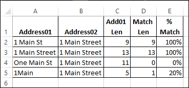
Here's a sample list, where the addresses in column A and B and being compared.

这是一个示例列表，其中将比较A和B列中的地址。

获取文本长度 (Get the Text Length)

The first step in calculating the percent that the cells match is to find the length of the address in column A. This formula is in cell C2:

计算单元格匹配百分比的第一步是在A列中找到地址的长度。此公式位于单元格C2中：

• =LEN(A2)

  = LEN(A2)

获取比赛长度 (Get the Match Length)

The formula in column D is doing the hard work. It finds how many characters, starting from the left in each cell, are a match. Lower and upper case are not compared.

D列中的公式正在进行艰苦的工作。 它查找从每个单元格的左侧开始有多少个字符匹配。 不比较大小写。

• =SUMPRODUCT( --(LEFT(A3, ROW(INDIRECT("A1:A" & C3))) =LEFT(B3, ROW(INDIRECT("A1:A" &C3)))))

  = SUMPRODUCT(-(LEFT(A3，ROW(INDIRECT(“ A1：A”＆C3))))= LEFT(B3，ROW(INDIRECT(“ A1：A”＆C3))))))

火柴公式如何工作 (How the Match Len Formula Works)

The INDIRECT function creates a reference to a range of cells, starting from cell A1. The range ends in column A, in the row that matches the length calculated in column C. So, in row 2, that range is A1:A9.

INDIRECT函数创建对从单元格A1开始的一系列单元格的引用。 范围在与列C中计算的长度匹配的行中的A列结束。因此，在第2行中，该范围为A1：A9。

The ROW function returns the row for each of the rows in that range. That's why we use ROW/INDIRECT, instead of just referring to the length in cell C2.

ROW函数返回该范围内每一行的行 。 这就是为什么我们使用ROW / INDIRECT而不是仅引用单元格C2中的长度的原因。

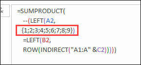
In this screen shot, I've used the F9 key to calculate that part of the formula, and you can see the row numbers.

在此屏幕快照中，我使用F9键来计算公式的该部分，您可以看到行号。

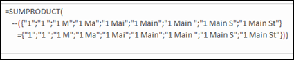
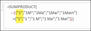
Then, the LEFT functions return the characters that are 1, 2, 3…characters to the left in each cell. In this screen shot, I've calculated both of the LEFT functions, and you can see that there is a match for lengths 1 through 9.

然后，LEFT函数将每个单元格左侧的1、2、3…个字符返回。 在此屏幕快照中，我已经计算了两个LEFT函数，并且可以看到长度1到9匹配。

However, if I do the same thing in row 5, only the first character is a match. After that, the characters are different in the two cells.

但是，如果我在第5行做同样的事情，则只有第一个字符是匹配项。 之后，两个单元格中的字符不同。

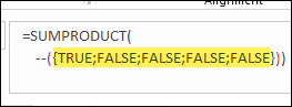
The equal sign compares the values for characters 1 through 5 in this example, and returns TRUE if they match, and FALSE if they do not match.

在此示例中，等号比较字符1到5的值，如果匹配则返回TRUE，否则返回FALSE。

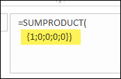
The double minus sign converts each TRUE to a 1, and each FALSE to a zero.

双减号将每个TRUE转换为1，将每个FALSE转换为零。

Finally, the SUMPRODUCT function adds up those numbers, to give the number of characters, from the left, that match. In row 5, that total is 1

最后， SUMPRODUCT函数将这些数字加起来，以从左侧给出匹配的字符数。 在第5行中，总数为1

获得百分比匹配 (Get the Percent Match)

Once the length and match length have been calculated, it's easy to find the percent matched. This formula is in cell E2, to compare the lengths:

一旦计算出长度和匹配长度，就很容易找到匹配百分比。 此公式在单元格E2中，以比较长度：

• =D2/C2

  = D2 / C2

There is a 100% match in row 2, and only a 20% match, starting from the left, in row 5.

第2行有100％的匹配，从第5行的左侧开始只有20％的匹配。

Thanks, UniMord, for sharing your formula to compare two cells, character by character.

感谢UniMord，感谢您共享公式来逐个字符地比较两个单元格。

比较两个单元格的更多方法 (More Ways to Compare Two Cells)

Here are a few more articles that show examples of how to compare two cells – either the full content, or partial content.

这里还有其他几篇文章，展示了如何比较两个单元格(全部内容还是部分内容)的示例。

• Use INDEX, MATCH and COUNTIF to find codes within text strings. There are other formulas in the comments too, so check those out.

  使用INDEX，MATCH和COUNTIF 在文本字符串中查找代码 。 注释中还有其他公式，因此请检查一下。

• Compare formulas on different sheets, with the FORMULATEXT and INDIRECT functions. Those functions are volatile though, so they'd slow down the workbook if you use too many of them.

  使用FORMULATEXT和INDIRECT函数比较不同工作表上的公式 。 这些功能是易变的，因此，如果您使用过多的功能，它们会使工作簿变慢。

• Be careful when using the Remove Duplicates feature in Excel – it treats real numbers and text numbers as the same value

  在Excel中使用“删除重复项”功能时要小心-它会将实数和文本数视为相同的值

翻译自: https://contexturesblog.com/archives/2018/04/12/how-to-compare-two-cells-in-excel/