谷歌浏览器网页表格复制一列_如何冻结或隐藏Google表格中的列和行

谷歌浏览器网页表格复制一列

The greater the number of rows and columns in your Google Sheets spreadsheet, the more unwieldy it can become. Freezing or hiding rows and columns can make your spreadsheet easier to read and navigate. Here’s how.

Google表格电子表格中的行和列越多，它变得越笨拙。 冻结或隐藏行和列可以使电子表格更易于阅读和浏览。 这是如何做。

冻结Google表格中的列和行 (Freeze Columns and Rows in Google Sheets)

If you freeze columns or rows in Google Sheets, it locks them into place. This is a good option for use with data-heavy spreadsheets, where you can freeze header rows or columns to make it easier to read your data.

如果冻结Google表格中的列或行，则会将其锁定到位。 这对于使用大量数据的电子表格来说是一个很好的选择，您可以在其中冻结标题行或列以使其更易于读取数据。

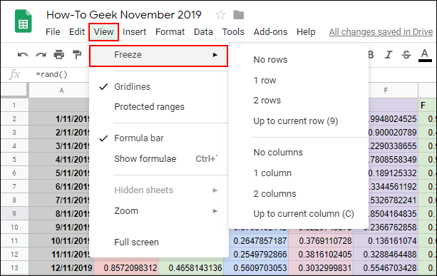
In most cases, you’ll want to freeze only the first row or column, but you can freeze rows or columns immediately after the first. To begin, select a cell in the column or row you’re looking to freeze and then click View > Freeze from the top menu.

在大多数情况下，您只想冻结第一行或第一列，但是可以在第一行或第一列之后立即冻结。 首先，在要冻结的列或行中选择一个单元格，然后从顶部菜单中单击查看>冻结。

Click “1 Column” or “1 Row” to freeze the top column A or row 1. Alternatively, click “2 Columns” or “2 Rows” to freeze the first two columns or rows.

单击“ 1列”或“ 1行”以冻结顶部的列A或行1。或者，单击“ 2列”或“ 2行”以冻结前两列或行。

You can also click “Up to Current Column” or “Up to Current Row” to freeze the columns or rows up to your selected cell.

您也可以单击“最多当前列”或“最多当前行”以冻结列或行，直到您选择的单元格。

When you move around your spreadsheet, your frozen cells will remain in place for you to easily refer back to.

当您在电子表格中四处移动时，冻结的单元格将保留在原处，以供您轻松参考。

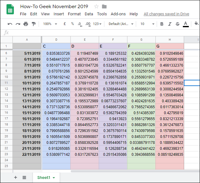
A thicker, gray cell border will appear next to a frozen column or row to make the border between your frozen and unfrozen cells clear.

冻结的列或行旁边会出现一个较粗的灰色单元格边框，以使冻结和未冻结的单元格之间的边界清晰可见。

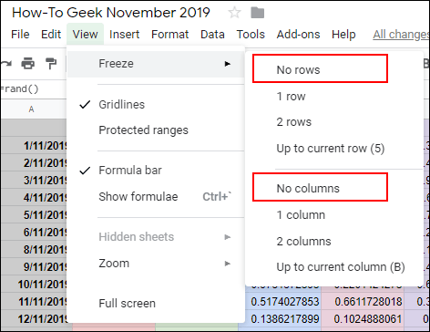
If you want to remove frozen columns or rows, click View > Frozen and select “No Rows” or “No Columns” to return these cells to normal.

如果要删除冻结的列或行，请单击“视图”>“冻结”，然后选择“无行”或“无列”以使这些单元格恢复正常。

隐藏Google表格中的列和行 (Hide Columns and Rows in Google Sheets)

If you want to temporarily hide certain rows or columns, but don’t want to remove them from your Google Sheets spreadsheet completely, you can hide them instead.

如果您要暂时隐藏某些行或列，但又不想将其完全从Google表格电子表格中删除，则可以将其隐藏。

隐藏Google表格列 (Hide Google Sheets Columns)

To hide a column, right-click the column header for your chosen column. In the menu that appears, click the “Hide Column” button.

要隐藏列，请右键单击所选列的列标题。 在出现的菜单中，单击“隐藏列”按钮。

Your column will then disappear from view, with arrows appearing in the column headers on either side of your hidden column.

然后，您的列将从视图中消失，隐藏的列两侧的列标题中都会出现箭头。

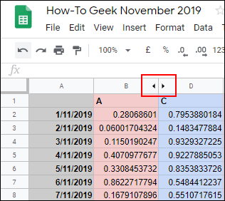
Clicking on these arrows will expose the column and return it to normal. Alternatively, you can use keyboard shortcuts in Google Sheets to hide your column instead.

单击这些箭头将显示该列并使其恢复正常。 或者，您可以使用Google表格中的键盘快捷键来隐藏列。

Click the column header to select it and then press Ctrl+Alt+0 on your keyboard to hide it instead. Selecting the columns on either side of your hidden row and then pressing Ctrl+Shift+0 on your keyboard will unhide your column afterward.

单击列标题以将其选中，然后按键盘上的Ctrl + Alt + 0使其隐藏。 选择隐藏行两边的列，然后按键盘上的Ctrl + Shift + 0将取消隐藏列。

隐藏Google表格行 (Hide Google Sheets Rows)

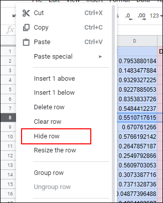
Similar to the process above, if you want to hide a row in Google Sheets, right-click on the row header for the row you’re looking to hide.

与上面的过程类似，如果要在Google表格中隐藏行，请右键单击要隐藏的行的行标题。

In the menu that appears, click the “Hide Row” button.

在出现的菜单中，单击“隐藏行”按钮。

Your selected row will disappear, with opposite arrows appearing in the header rows on either side.

您选择的行将消失，左右两边的标题行中将出现相反的箭头。

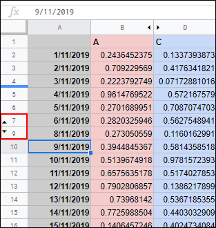
Click on these arrows to display your hidden row and return it to normal at any point.

单击这些箭头以显示隐藏的行，然后随时将其恢复为正常。

If you’d prefer to use a keyboard shortcut, click the row header to select it and then press Ctrl+Alt+9 to hide the row instead. Select the rows on either side of your hidden row and press Ctrl+Shift+9 on your keyboard to unhide it afterward.

如果您想使用键盘快捷键，请单击行标题以将其选中，然后按Ctrl + Alt + 9来隐藏该行。 选择隐藏行两侧的行，然后按键盘上的Ctrl + Shift + 9使其随后取消隐藏。

翻译自: https://www.howtogeek.com/446672/how-to-freeze-or-hide-columns-and-rows-in-google-sheets/

谷歌浏览器网页表格复制一列