


sql数据透视
In this article, in the series, we’ll discuss understanding and preparing data by using SQL unpivot.
在本系列文章中,我们将讨论使用SQL unpivot理解和准备数据。
As I announced in my previous article, Data science in SQL Server: pivoting and transposing data, this one is talking about the opposite process to pivoting, the unpivoting process. With unpivoting, you rotate the data to get rows from specific number of columns, with the original column names stored as a value in the rows of a new, unpivoted column. Unpivoting might be even more frequent operation in data science data preparation than pivoting because quite a lot of data exist in spreadsheets and other table formats that are not suitable for an immediate use.
正如我在上一篇文章《 SQL Server中的数据科学:数据透视和转置》中所宣布的那样,本文讨论的是与透视相反的过程,即不可透视的过程。 通过取消透视,您可以旋转数据以从特定数量的列中获取行,并将原始列名作为值存储在新的,未被透视的列的行中。 数据透视表中的数据透视表操作可能比数据透视表操作更为频繁,因为电子表格和其他不适合立即使用的表格式中存在大量数据。
Instead of any further explanation of unpivoting, I will show you the process through examples.
我将通过示例向您展示该过程,而不是对其进行任何进一步的解释。
T-SQL Unpivot运算符和其他可能性 (T-SQL Unpivot Operator and Other Possibilities)
As always, I need some data to work on. The following query creates a table with pivoted data.
和往常一样,我需要一些数据来处理。 以下查询创建一个包含数据透视表。
USE AdventureWorksDW2017;
GO
-- Data preparation - pivoting
WITH PCTE AS
(
SELECT g.EnglishCountryRegionName AS Country,
 d.CalendarYear AS CYear,
 SUM(s.SalesAmount) AS Sales
FROM dbo.FactInternetSales s
 INNER JOIN dbo.DimDate d
  ON d.DateKey = s.OrderDateKey
 INNER JOIN dbo.DimCustomer c
  ON c.CustomerKey = s.CustomerKey
 INNER JOIN dbo.DimGeography g
  ON g.GeographyKey = c.GeographyKey
WHERE g.EnglishCountryRegionName IN (N'Australia', N'Canada')
GROUP BY
 g.EnglishCountryRegionName,
 g.StateProvinceName,
 d.CalendarYear
)
SELECT Country, [2010], [2011], [2012], [2013], [2014]
INTO dbo.SalesPivoted
FROM PCTE
 PIVOT (SUM(Sales) FOR CYear
    IN ([2010], [2011], [2012], [2013], [2014])) AS P;
GO
The following query checks the content of the table I just created.
以下查询检查我刚刚创建的表的内容。
SELECT Country, [2010], [2011], [2012], [2013], [2014]
FROM dbo.SalesPivoted;
Here is the result, the pivoted table:
结果是数据透视表:
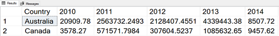
In a data science projects, you might have a task to forecast the sales over countries and years. You need to create time series, with years as time points. Since you have data for five years in five columns, you need to create five rows for each year. You will get five rows per country, with a new column that denotes the year, with the original column names [2010] to [2014] as the values of this new column. You will get another new column with sales data. The values of this column will be the respective values of the cells in the intersection of each country with each year. For example, the for the row with country Australia and year 2010, the sales value will be 20,909.78. My first query uses the T-SQL UNPIVOT operator.
在数据科学项目中,您可能需要预测国家和地区的销售额。 您需要创建以年为时间点的时间序列。 由于您有五个列中的五年数据,因此您需要每年创建五行。 每个国家/地区您将获得五行,其中有一个新列表示年份,原始列名[2010]至[2014]是该新列的值。 您将获得另一个包含销售数据的新列。 此列的值将是每个国家/地区与每年相交的单元格的相应值。 例如,与国家(地区)澳大利亚和2010年的行的销售价值将为20,909.78。 我的第一个查询使用T-SQL UNPIVOT运算符。
SELECT Country, CYear, Sales
FROM dbo.SalesPivoted
  UNPIVOT(Sales FOR CYear
          IN ([2010], [2011], [2012], [2013], [2014])) AS U
ORDER BY Country, CYear;
Here is the unpivoted result. You can see that I used the name CYear for the year column (denoting calendar year) and Sales for the value column:
这是无懈可击的结果。 您可以看到,我在年列(表示日历年)中使用了CYear,在值列中使用了Sales:

Similarly like the PIVOT operator, the UNPIVOT operator is also not a part of the ANSI SQL standard. In order to have your data science project code prepared for multiple database management systems, you might want to use the standard ANSI SQL expressions only. For each original row, for each country, you have to create five rows, one for each year. You can do it with a cross join of the original table with the tabular expression in the FROM clause that returns the five rows. Then you use the CASE expression to extract the correct value for each year. Finally, you need to eliminate rows with unknown sales. This last task is just to have completely the same logic as the PIVOT operator, which eliminates rows with NULLs in the value column. In your data science project, you might keep NULLs, and replace them with some default value, in order to have all time points present. Note that in the demo dataset I am using, there are no NULLs, so the result of the following query would be the same even without the WHERE clause.
与PIVOT运算符类似,UNPIVOT运算符也不是ANSI SQL标准的一部分。 为了为多个数据库管理系统准备数据科学项目代码,您可能只想使用标准的ANSI SQL表达式。 对于每个原始行,对于每个国家/地区,您都必须创建五行,每年一行。 您可以通过将原始表与返回五行的FROM子句中的表格表达式进行交叉联接来实现。 然后,您可以使用CASE表达式提取每年的正确值。 最后,您需要消除销量未知的行。 最后一项任务是拥有与PIVOT运算符完全相同的逻辑,该运算符消除了value列中带有NULL的行。 在您的数据科学项目中,您可以保留NULL,然后将其替换为某些默认值,以便显示所有时间点。 请注意,在我正在使用的演示数据集中,没有NULL,因此即使没有WHERE子句,以下查询的结果也将相同。
SELECT Country, CYear, Sales
FROM
 (SELECT Country, CYear,
   CASE CYear
     WHEN 2010 THEN [2010]
     WHEN 2011 THEN [2011]
     WHEN 2012 THEN [2012]
     WHEN 2013 THEN [2013]
     WHEN 2014 THEN [2014]
   END AS Sales
  FROM dbo.SalesPivoted
   CROSS JOIN (
    SELECT 2010 AS CYear
    UNION ALL SELECT 2011
    UNION ALL SELECT 2012
    UNION ALL SELECT 2013
    UNION ALL SELECT 2014) AS CY) AS D
WHERE Sales IS NOT NULL
ORDER BY Country, CYear;
In T-SQL, you could also use the CROSS APPLY operator to apply a tabular expression for each row from the original table. You can also create the five rows, one for each year, with the VALUES clause, which is a shorthand for multiple SELECT … UNION clauses. Like the following example shows, the query becomes shorter.
在T-SQL中,您还可以使用CROSS APPLY运算符为原始表中的每一行应用表格表达式。 您还可以使用VALUES子句创建五行,每行一年,这是多个SELECT…UNION子句的简写。 如以下示例所示,查询变得更短。
SELECT Country, CYear, Sales
FROM dbo.SalesPivoted
 CROSS APPLY (
  VALUES (2010, [2010]),
         (2011, [2011]),
         (2012, [2012]),
         (2013, [2013]),
         (2014, [2014])
  ) AS U( CYear, Sales )
WHERE Sales IS NOT NULL
ORDER BY Country, CYear;
However, the APPLY operator is also a T-SQL extension of the ANSI standard. You might still prefer to use the standard SQL in your projects.
但是,APPLY运算符也是ANSI标准的T-SQL扩展。 您可能仍希望在项目中使用标准SQL。
In all of the queries so far, I had to write manually the list of the values for the CYear column. Therefore, you can unpivot only a fixed number of original columns. The question is, of course, can you create this list dynamically, as I have shown in my previous article for the PIVOT operator. And the answer is yes. All you need to know is that in SQL Server, you can find all column names of all tables in sys.columns catalog view. Then you can use the STRING_AGG() function to get a delimited list of the column names.
到目前为止,在所有查询中,我都必须手动编写CYear列的值列表。 因此,您只能取消固定数目的原始列。 当然,问题是,您能否动态创建此列表,就像我在上一篇文章中为PIVOT运算符所显示的那样。 答案是肯定的。 您需要知道的是,在SQL Server中,您可以在sys.columns目录视图中找到所有表的所有列名称。 然后,您可以使用STRING_AGG()函数获取列名的分隔列表。
DECLARE @stmtvar AS NVARCHAR(4000);
SET @stmtvar = N'
SELECT Country, CYear, Sales
FROM dbo.SalesPivoted
  UNPIVOT(Sales FOR CYear
          IN ('
+
(SELECT STRING_AGG(QUOTENAME([name]), N', ')
        WITHIN GROUP (ORDER BY [name])
 FROM
 (
 SELECT [name]
 FROM sys.columns
 WHERE object_id = OBJECT_ID(N'dbo.SalesPivoted', N'U')
   AND name LIKE N'2%'
 ) AS Y)
+ N')) AS U
ORDER BY Country, CYear;';
EXEC sys.sp_executesql @stmt = @stmtvar;
GO
It is time to switch to the languages that are more oriented towards data science.
现在该切换到更面向数据科学的语言了。
取消枢纽 (Unpivoting in R)
Let me read the pivoted data from SQL Server in R.
让我从R中SQL Server中读取透视数据。
library(RODBC)
con <- odbcConnect("AWDW", uid = "RUser", pwd = "Pa$$w0rd")
SGY <- as.data.frame(sqlQuery(con,
   "SELECT Country, [2010], [2011], [2012], [2013], [2014]
    FROM dbo.SalesPivoted;"),
    stringsAsFactors = TRUE)
close(con)
View(SGY)
You can use the stack() function from the basic installation to unpivot the data. The following code stacks vertically the data from the SGY data frame without the first column.
您可以使用基本安装中的stack()函数取消数据透视。 以下代码垂直堆叠来自SGY数据帧的数据,而没有第一列。
stack(SGY[-1])
Here is the result:
结果如下:
| values | ind | |
| 1 | 20909.78 | 2010 |
| 2 | 3578.27 | 2010 |
| 3 | 2563732.25 | 2011 |
| 4 | 571571.80 | 2011 |
| 5 | 2128407.46 | 2012 |
| 6 | 307604.52 | 2012 |
| 7 | 4339443.38 | 2013 |
| 8 | 1085632.65 | 2013 |
| 9 | 8507.72 | 2014 |
| 10 | 9457.62 | 2014 |
| 价值观 | 印 | |
| 1个 | 20909.78 | 2010 |
| 2 | 3578.27 | 2010 |
| 3 | 2563732.25 | 2011年 |
| 4 | 571571.80 | 2011年 |
| 5 | 2128407.46 | 2012年 |
| 6 | 307604.52 | 2012年 |
| 7 | 4339443.38 | 2013年 |
| 8 | 1085632.65 | 2013年 |
| 9 | 8507.72 | 2014年 |
| 10 | 9457.62 | 2014年 |
You can see that I lost the country values. I can add them back with the following code.
您可以看到我失去了国家价值观。 我可以使用以下代码将其添加回去。
cbind(rbind(SGY[1], SGY[1], SGY[1], SGY[1], SGY[1]), stack(SGY[-1]))
In the previous code, I used the rbind() function to multiply the first two rows of the original data frame with the first column only, with the country only. Now I have ten rows, which I can bind as a new column with the cbind() function to the result of the stack() function. Here is the result:
在前面的代码中,我使用rbind()函数将原始数据帧的前两行与第一列(仅与国家/地区)相乘。 现在,我有十行,可以使用cbind()函数将其绑定为stack()函数的结果作为新列。 结果如下:
Country 国家 values 价值观 ind 印 1 1个 Australia 澳大利亚 20909.78 20909.78 2010 2010 2 2 Canada 加拿大 3578.27 3578.27 2010 2010 3 3 Australia 澳大利亚 2563732.25 2563732.25 2011 2011年 4 4 Canada 加拿大 571571.80 571571.80 2011 2011年 5 5 Australia 澳大利亚 2128407.46 2128407.46 2012 2012年 6 6 Canada 加拿大 307604.52 307604.52 2012 2012年 7 7 Australia 澳大利亚 4339443.38 4339443.38 2013 2013年 8 8 Canada 加拿大 1085632.65 1085632.65 2013 2013年 9 9 Australia 澳大利亚 8507.72 8507.72 2014 2014年 10 10 Canada 加拿大 9457.62 9457.62 2014 2014年This was not a very useful code. Besides adding the countries manually, I also did not change the default column names for the two new columns, the values and the column.
这不是一个非常有用的代码。 除了手动添加国家/地区之外,我也没有更改两个新列(值和列)的默认列名。
To make the complete unpivoting dynamically, I can use the melt() function from the reshape package. Here is an example.
为了使整个动态动态完成,我可以使用reshape包中的melt()函数。 这是一个例子。
library(reshape)
SU <- melt(SGY, id = c("Country"))
SU
The following result shows that I still have default names for them to new columns. The melt() function assigns the names variable and value. In addition, I didn’t care about the order of the rows.
以下结果表明,对于新列,我仍然具有默认名称。 melt()函数分配名称变量和值。 另外,我不在乎行的顺序。
| Country | variable | value | |
| 1 | Australia | 2010 | 20909.78 |
| 2 | Canada | 2010 | 3578.27 |
| 3 | Australia | 2011 | 2563732.25 |
| 4 | Canada | 2011 | 571571.80 |
| 5 | Australia | 2012 | 2128407.46 |
| 6 | Canada | 2012 | 307604.52 |
| 7 | Australia | 2013 | 4339443.38 |
| 8 | Canada | 2013 | 1085632.65 |
| 9 | Australia | 2014 | 8507.72 |
| 10 | Canada | 2014 | 9457.62 |
| 国家 | 变量 | 值 | |
| 1个 | 澳大利亚 | 2010 | 20909.78 |
| 2 | 加拿大 | 2010 | 3578.27 |
| 3 | 澳大利亚 | 2011年 | 2563732.25 |
| 4 | 加拿大 | 2011年 | 571571.80 |
| 5 | 澳大利亚 | 2012年 | 2128407.46 |
| 6 | 加拿大 | 2012年 | 307604.52 |
| 7 | 澳大利亚 | 2013年 | 4339443.38 |
| 8 | 加拿大 | 2013年 | 1085632.65 |
| 9 | 澳大利亚 | 2014年 | 8507.72 |
| 10 | 加拿大 | 2014年 | 9457.62 |
I will take care of the column names and the row order with the rename() and arrange() functions from the dplyr package.
我将使用dplyr包中的rename()和ranging()函数来处理列名和行顺序。
library(dplyr)
SUO <-
rename(SU, CYear = variable, Sales = value) %>%
arrange(Country, CYear)
SUO
Now I got the result I wanted.
现在我得到了想要的结果。
| Country | CYear | Sales | |
| 1 | Australia | 2010 | 20909.78 |
| 2 | Australia | 2011 | 2563732.25 |
| 3 | Australia | 2012 | 2128407.46 |
| 4 | Australia | 2013 | 4339443.38 |
| 5 | Australia | 2014 | 8507.72 |
| 6 | Canada | 2010 | 3578.27 |
| 7 | Canada | 2011 | 571571.80 |
| 8 | Canada | 2012 | 307604.52 |
| 9 | Canada | 2013 | 1085632.65 |
| 10 | Canada | 2014 | 9457.62 |
| 国家 | 循环 | 营业额 | |
| 1个 | 澳大利亚 | 2010 | 20909.78 |
| 2 | 澳大利亚 | 2011年 | 2563732.25 |
| 3 | 澳大利亚 | 2012年 | 2128407.46 |
| 4 | 澳大利亚 | 2013年 | 4339443.38 |
| 5 | 澳大利亚 | 2014年 | 8507.72 |
| 6 | 加拿大 | 2010 | 3578.27 |
| 7 | 加拿大 | 2011年 | 571571.80 |
| 8 | 加拿大 | 2012年 | 307604.52 |
| 9 | 加拿大 | 2013年 | 1085632.65 |
| 10 | 加拿大 | 2014年 | 9457.62 |
I will show one more option in R – the gather() function from the tidyr package. I can define the new column names when calling this function directly. Then I can use the arrange() function again to sort the data, like the following code shows. The result is the same as above.
我将在R中显示另一个选项– tidyr包中的collect()函数。 直接调用此函数时,可以定义新的列名。 然后,我可以再次使用ranging()函数对数据进行排序,如以下代码所示。 结果与上面相同。
library(tidyr)
gather(SGY, key = CYear, value = Sales, - Country) %>%
arrange(Country, CYear)
Time to show another graph. This time, I am using the plot_ly() function from the plotly library. With this library, you can make interactive graphs online. Therefore, the next graph opens in a Web browser.
是时候显示另一个图形了。 这次,我正在使用plotly库中的plot_ly()函数。 使用此库,您可以在线制作交互式图形。 因此,下一个图形将在Web浏览器中打开。
library(plotly)
plot_ly(data = SUO, labels = ~SUO$Country, values = ~SUO$Sales) %>%
  add_pie(hole = 0.6) %>%
  layout(title = "Sales by Country", showlegend = T,
         xaxis = list(showgrid = FALSE, zeroline = FALSE, showticklabels = FALSE),
         yaxis = list(showgrid = FALSE, zeroline = FALSE, showticklabels = FALSE))
Here is the plotly graph, showing the sales oved countries in a donut chart:
这是一个绘图图,以甜甜圈图显示了销售国家/地区:
In the next section, I will show how to do the unpivoting in Python.
在下一节中,我将展示如何在Python中进行取消透视。
Python熊猫透视 (Python Pandas Unpivoting)
Let me again start with imports and with reading the data from SQL Server.
让我再次从导入和从SQL Server读取数据开始。
import numpy as np
import pandas as pd
import pyodbc
import matplotlib.pyplot as plt
# Connecting and reading the data
con = pyodbc.connect('DSN=AWDW;UID=RUser;PWD=Pa$$w0rd')
query = """
SELECT Country, [2010], [2011], [2012], [2013], [2014]
FROM dbo.SalesPivoted;"""
SGY = pd.read_sql(query, con)
SGY.head()
I will find all methods I need for unpivoting in the pandas library. The first method I am showing is the unstack() method.
我将在pandas库中找到取消透视所需的所有方法。 我展示的第一个方法是unstack()方法。
SGY.unstack()
Here is the result:
结果如下:
| Country | 0 | Australia |
| 1 | Canada | |
| 2010 | 0 | 20909.8 |
| 1 | 3578.27 | |
| 2011 | 0 | 2.56373e+06 |
| 1 | 571572 | |
| 2012 | 0 | 2.12841e+06 |
| 1 | 307605 | |
| 2013 | 0 | 4.33944e+06 |
| 1 | 1.08563e+06 | |
| 2014 | 0 | 8507.72 |
| 1 | 9457.62 |
| 国家 | 0 | 澳大利亚 |
| 1个 | 加拿大 | |
| 2010 | 0 | 20909.8 |
| 1个 | 3578.27 | |
| 2011年 | 0 | 2.56373e + 06 |
| 1个 | 571572 | |
| 2012年 | 0 | 2.12841e + 06 |
| 1个 | 307605 | |
| 2013年 | 0 | 4.33944e + 06 |
| 1个 | 1.08563e + 06 | |
| 2014年 | 0 | 8507.72 |
| 1个 | 9457.62 |
I got a two-level index or a multi-index. I can use the rest_index() method to get flattened index structure with both levels shown explicitly, like the following code shows.
我有两级索引或多级索引。 我可以使用rest_index()方法来获取扁平化的索引结构,同时明确显示两个级别,如以下代码所示。
SGY.unstack().reset_index(name = 'Sales')
Here is the result:
结果如下:
| Level 0 | Level 1 | Sales | |
| 0 | Country | 0 | Australia |
| 1 | Country | 1 | Canada |
| 2 | 2010 | 0 | 20909.8 |
| 3 | 2010 | 1 | 3578.27 |
| 4 | 2011 | 0 | 2.56373e+06 |
| 5 | 2011 | 1 | 571572 |
| 6 | 2012 | 0 | 2.12841e+06 |
| 7 | 2012 | 1 | 307605 |
| 8 | 2013 | 0 | 4.33944e+06 |
| 9 | 2013 | 1 | 1.08563e+06 |
| 10 | 2014 | 0 | 8507.72 |
| 11 | 2014 | 1 | 9457.62 |
| 0级 | 1级 | 营业额 | |
| 0 | 国家 | 0 | 澳大利亚 |
| 1个 | 国家 | 1个 | 加拿大 |
| 2 | 2010 | 0 | 20909.8 |
| 3 | 2010 | 1个 | 3578.27 |
| 4 | 2011年 | 0 | 2.56373e + 06 |
| 5 | 2011年 | 1个 | 571572 |
| 6 | 2012年 | 0 | 2.12841e + 06 |
| 7 | 2012年 | 1个 | 307605 |
| 8 | 2013年 | 0 | 4.33944e + 06 |
| 9 | 2013年 | 1个 | 1.08563e + 06 |
| 10 | 2014年 | 0 | 8507.72 |
| 11 | 2014年 | 1个 | 9457.62 |
Still, the result is not very useful. The melt() function returns a more standard data frame result.
尽管如此,结果仍然不是很有用。 melt()函数返回更标准的数据帧结果。
pd.melt(SGY, id_vars = ['Country'])
You can see the output of the melt() function bellow:
您可以在下面看到melt()函数的输出:
| Country | variable | value | |
| 0 | Australia | 2010 | 2.090978e+04 |
| 1 | Canada | 2010 | 3.578270e+03 |
| 2 | Australia | 2011 | 2.563732e+06 |
| 3 | Canada | 2011 | 5.715718e+05 |
| 4 | Australia | 2012 | 2.128407e+06 |
| 5 | Canada | 2012 | 3.076045e+05 |
| 6 | Australia | 2013 | 4.339443e+06 |
| 7 | Canada | 2013 | 1.085633e+06 |
| 8 | Australia | 2014 | 8.507720e+03 |
| 9 | Canada | 2014 | 9.457620e+03 |
| 国家 | 变量 | 值 | |
| 0 | 澳大利亚 | 2010 | 2.090978e + 04 |
| 1个 | 加拿大 | 2010 | 3.578270e + 03 |
| 2 | 澳大利亚 | 2011年 | 2.563732e + 06 |
| 3 | 加拿大 | 2011年 | 5.715718e + 05 |
| 4 | 澳大利亚 | 2012年 | 2.128407e + 06 |
| 5 | 加拿大 | 2012年 | 3.076045e + 05 |
| 6 | 澳大利亚 | 2013年 | 4.339443e + 06 |
| 7 | 加拿大 | 2013年 | 1.085633e + 06 |
| 8 | 澳大利亚 | 2014年 | 8.507720e + 03 |
| 9 | 加拿大 | 2014年 | 9.457620e + 03 |
Finally, let me also rename the columns and sort the data.
最后,让我也重命名列并对数据进行排序。
SUO = pd.melt(SGY, id_vars = ['Country'],
        var_name = 'CYear',
        value_name = 'Sales').sort_values(by = ['Country', 'CYear'])
SUO
The next result is again in the form I wanted to achieve.
下一个结果还是我想要实现的形式。
| Country | CYear | Sales | |
| 1 | Australia | 2010 | 2.090978e+04 |
| 2 | Australia | 2011 | 2.563732e+06 |
| 3 | Australia | 2012 | 2.128407e+06 |
| 4 | Australia | 2013 | 4.339443e+06 |
| 5 | Australia | 2014 | 8.507720e+03 |
| 6 | Canada | 2010 | 3.578270e+03 |
| 7 | Canada | 2011 | 5.715718e+05 |
| 8 | Canada | 2012 | 3.076045e+05 |
| 9 | Canada | 2013 | 1.085633e+06 |
| 10 | Canada | 2014 | 9.457620e+03 |
| 国家 | 循环 | 营业额 | |
| 1个 | 澳大利亚 | 2010 | 2.090978e + 04 |
| 2 | 澳大利亚 | 2011年 | 2.563732e + 06 |
| 3 | 澳大利亚 | 2012年 | 2.128407e + 06 |
| 4 | 澳大利亚 | 2013年 | 4.339443e + 06 |
| 5 | 澳大利亚 | 2014年 | 8.507720e + 03 |
| 6 | 加拿大 | 2010 | 3.578270e + 03 |
| 7 | 加拿大 | 2011年 | 5.715718e + 05 |
| 8 | 加拿大 | 2012年 | 3.076045e + 05 |
| 9 | 加拿大 | 2013年 | 1.085633e + 06 |
| 10 | 加拿大 | 2014年 | 9.457620e + 03 |
And for the last thing, let me show the sales over years for both countries together in a pandas area chart.
最后,让我在熊猫面积图中共同显示这两个国家多年来的销售额。
SUO.plot(kind = 'area', y = 'Sales', x = 'CYear')
plt.show()
The following figure shows the graph:
下图显示了该图:
结论 (Conclusion)
I am done with pivoting and unpivoting. However, I am not done with the data preparation yet. So far, I always had a dataset with known values only. What happens if there are NULLs in the data? Stay tuned for the forthcoming articles.
我已经完成了透视和透视。 但是,我还没有完成数据准备工作。 到目前为止,我始终只有一个具有已知值的数据集。 如果数据中有NULL,该怎么办? 请继续关注即将发表的文章。
目录 (Table of contents)
资料下载 (Downloads)
- Data Science in SQL Server Unpivoting Data_CodeSQL Server中的数据科学取消数据_代码
- Data Science in SQL Server Unpivoting Data_FiguresSQL Server中的数据科学取消数据透视图
翻译自: https://www.sqlshack.com/data-science-in-sql-server-unpivoting-data/
sql数据透视


 1443
1443


 被折叠的 条评论
为什么被折叠?
被折叠的 条评论
为什么被折叠?
 到【灌水乐园】发言


