


TensorFlow-快速指南 (TensorFlow - Quick Guide)
TensorFlow-简介 (TensorFlow - Introduction)
TensorFlow is a software library or framework, designed by the Google team to implement machine learning and deep learning concepts in the easiest manner. It combines the computational algebra of optimization techniques for easy calculation of many mathematical expressions.
TensorFlow是Google团队设计的软件库或框架,用于以最简单的方式实现机器学习和深度学习的概念。 它结合了优化技术的计算代数,可轻松计算许多数学表达式。
The official website of TensorFlow is mentioned below −
TensorFlow的官方网站如下-

Let us now consider the following important features of TensorFlow −
现在让我们考虑TensorFlow的以下重要功能-
It includes a feature of that defines, optimizes and calculates mathematical expressions easily with the help of multi-dimensional arrays called tensors.
它具有的一项功能是借助称为张量的多维数组轻松定义,优化和计算数学表达式。
It includes a programming support of deep neural networks and machine learning techniques.
它包括对深度神经网络和机器学习技术的编程支持。
It includes a high scalable feature of computation with various data sets.
它包括具有各种数据集的高度可扩展的计算功能。
TensorFlow uses GPU computing, automating management. It also includes a unique feature of optimization of same memory and the data used.
TensorFlow使用GPU计算,实现了自动化管理。 它还具有优化相同内存和所用数据的独特功能。
为什么TensorFlow如此受欢迎? (Why is TensorFlow So Popular?)
TensorFlow is well-documented and includes plenty of machine learning libraries. It offers a few important functionalities and methods for the same.
TensorFlow有充分的文档证明,并包含大量的机器学习库。 它提供了一些重要的功能和方法。
TensorFlow is also called a “Google” product. It includes a variety of machine learning and deep learning algorithms. TensorFlow can train and run deep neural networks for handwritten digit classification, image recognition, word embedding and creation of various sequence models.
TensorFlow也被称为“ Google”产品。 它包括各种机器学习和深度学习算法。 TensorFlow可以训练和运行深度神经网络,以进行手写数字分类,图像识别,单词嵌入和创建各种序列模型。
TensorFlow-安装 (TensorFlow - Installation)
To install TensorFlow, it is important to have “Python” installed in your system. Python version 3.4+ is considered the best to start with TensorFlow installation.
要安装TensorFlow,在系统中安装“ Python”非常重要。 从TensorFlow安装开始,Python 3.4+被认为是最好的选择。
Consider the following steps to install TensorFlow in Windows operating system.
考虑以下步骤在Windows操作系统中安装TensorFlow。
Step 1 − Verify the python version being installed.
步骤1-验证正在安装的python版本。

Step 2 − A user can pick up any mechanism to install TensorFlow in the system. We recommend “pip” and “Anaconda”. Pip is a command used for executing and installing modules in Python.
步骤2-用户可以选择任何机制在系统中安装TensorFlow。 我们建议使用“点子”和“ Anaconda”。 Pip是用于在Python中执行和安装模块的命令。
Before we install TensorFlow, we need to install Anaconda framework in our system.
在安装TensorFlow之前,我们需要在系统中安装Anaconda框架。

After successful installation, check in command prompt through “conda” command. The execution of command is displayed below −
成功安装后,通过“ conda”命令检入命令提示符。 命令的执行如下所示-

Step 3 − Execute the following command to initialize the installation of TensorFlow −
步骤3-执行以下命令以初始化TensorFlow的安装-
conda create --name tensorflow python = 3.5

It downloads the necessary packages needed for TensorFlow setup.
它下载TensorFlow设置所需的必要软件包。
Step 4 − After successful environmental setup, it is important to activate TensorFlow module.
步骤4-成功设置环境后,激活TensorFlow模块很重要。
activate tensorflow

Step 5 − Use pip to install “Tensorflow” in the system. The command used for installation is mentioned as below −
步骤5-使用pip在系统中安装“ Tensorflow”。 用于安装的命令如下所述-
pip install tensorflow
And,
和,
pip install tensorflow-gpu


After successful installation, it is important to know the sample program execution of TensorFlow.
成功安装后,了解TensorFlow的示例程序执行非常重要。
Following example helps us understand the basic program creation “Hello World” in TensorFlow.
以下示例可帮助我们了解TensorFlow中的基本程序创建“ Hello World”。

The code for first program implementation is mentioned below −
下面提到了第一个程序实现的代码-
>> activate tensorflow
>> python (activating python shell)
>> import tensorflow as tf
>> hello = tf.constant(‘Hello, Tensorflow!’)
>> sess = tf.Session()
>> print(sess.run(hello))
了解人工智能 (Understanding Artificial Intelligence)
Artificial Intelligence includes the simulation process of human intelligence by machines and special computer systems. The examples of artificial intelligence include learning, reasoning and self-correction. Applications of AI include speech recognition, expert systems, and image recognition and machine vision.
人工智能包括通过机器和专用计算机系统进行的人类仿真过程。 人工智能的例子包括学习,推理和自我纠正。 AI的应用包括语音识别,专家系统以及图像识别和机器视觉。
Machine learning is the branch of artificial intelligence, which deals with systems and algorithms that can learn any new data and data patterns.
机器学习是人工智能的分支,它处理可以学习任何新数据和数据模式的系统和算法。
Let us focus on the Venn diagram mentioned below for understanding machine learning and deep learning concepts.
让我们专注于下面提到的维恩图,以了解机器学习和深度学习的概念。

Machine learning includes a section of machine learning and deep learning is a part of machine learning. The ability of program which follows machine learning concepts is to improve its performance of observed data. The main motive of data transformation is to improve its knowledge in order to achieve better results in the future, provide output closer to the desired output for that particular system. Machine learning includes “pattern recognition” which includes the ability to recognize the patterns in data.
机器学习包括机器学习的一部分,而深度学习是机器学习的一部分。 遵循机器学习概念的程序的能力是提高其观测数据的性能。 数据转换的主要动机是提高其知识水平,以便将来获得更好的结果,为特定系统提供更接近所需输出的输出。 机器学习包括“模式识别”,其中包括识别数据中模式的能力。
The patterns should be trained to show the output in desirable manner.
模式应经过训练以期望的方式显示输出。
Machine learning can be trained in two different ways −
机器学习可以两种不同的方式进行训练-
- Supervised training 有监督的培训
- Unsupervised training 无监督培训
监督学习 (Supervised Learning)
Supervised learning or supervised training includes a procedure where the training set is given as input to the system wherein, each example is labeled with a desired output value. The training in this type is performed using minimization of a particular loss function, which represents the output error with respect to the desired output system.
监督学习或监督训练包括以下过程:将训练集作为系统的输入,其中,每个示例都标有所需的输出值。 使用特定损失函数的最小化来执行这种类型的训练,该损失函数表示相对于所需输出系统的输出误差。
After completion of training, the accuracy of each model is measured with respect to disjoint examples from training set, also called the validation set.
训练完成后,针对训练集(也称为验证集)中不相交的示例,测量每个模型的准确性。

The best example to illustrate “Supervised learning” is with a bunch of photos given with information included in them. Here, the user can train a model to recognize new photos.
举例说明“监督学习”的最好例子是一堆照片,其中包含信息。 在这里,用户可以训练模型以识别新照片。
无监督学习 (Unsupervised Learning)
In unsupervised learning or unsupervised training, include training examples, which are not labeled by the system to which class they belong. The system looks for the data, which share common characteristics, and changes them based on internal knowledge features.This type of learning algorithms are basically used in clustering problems.
在无监督学习或无监督培训中,请包括培训示例,这些示例未按其所属的系统标记。 该系统寻找具有共同特征的数据,并根据内部知识特征对其进行更改。这种学习算法基本上用于聚类问题。
The best example to illustrate “Unsupervised learning” is with a bunch of photos with no information included and user trains model with classification and clustering. This type of training algorithm works with assumptions as no information is given.
最好的例子来说明“无监督学习”是一堆没有信息的照片,以及带有分类和聚类的用户训练模型。 由于没有给出任何信息,因此这种训练算法可以在假设条件下使用。

TensorFlow-数学基础 (TensorFlow - Mathematical Foundations)
It is important to understand mathematical concepts needed for TensorFlow before creating the basic application in TensorFlow. Mathematics is considered as the heart of any machine learning algorithm. It is with the help of core concepts of Mathematics, a solution for specific machine learning algorithm is defined.
在TensorFlow中创建基本应用程序之前,了解TensorFlow所需的数学概念非常重要。 数学被视为任何机器学习算法的核心。 借助于数学的核心概念,定义了针对特定机器学习算法的解决方案。
向量 (Vector)
An array of numbers, which is either continuous or discrete, is defined as a vector. Machine learning algorithms deal with fixed length vectors for better output generation.
连续或离散的数字数组被定义为向量。 机器学习算法处理固定长度的向量,以产生更好的输出。
Machine learning algorithms deal with multidimensional data so vectors play a crucial role.
机器学习算法处理多维数据,因此向量起着至关重要的作用。

The pictorial representation of vector model is as shown below −
向量模型的图形表示如下所示-

标量 (Scalar)
Scalar can be defined as one-dimensional vector. Scalars are those, which include only magnitude and no direction. With scalars, we are only concerned with the magnitude.
标量可以定义为一维向量。 标量是仅包含幅度而无方向的标量。 对于标量,我们只关心幅度。
Examples of scalar include weight and height parameters of children.
标量的示例包括孩子的体重和身高参数。
矩阵 (Matrix)
Matrix can be defined as multi-dimensional arrays, which are arranged in the format of rows and columns. The size of matrix is defined by row length and column length. Following figure shows the representation of any specified matrix.
矩阵可以定义为多维数组,以行和列的格式排列。 矩阵的大小由行长和列长定义。 下图显示了任何指定矩阵的表示形式。

Consider the matrix with “m” rows and “n” columns as mentioned above, the matrix representation will be specified as “m*n matrix” which defined the length of matrix as well.
考虑如上所述的具有“ m”行和“ n”列的矩阵,矩阵表示将被指定为“ m * n矩阵”,其也定义了矩阵的长度。
数学计算 (Mathematical Computations)
In this section, we will learn about the different Mathematical Computations in TensorFlow.
在本部分中,我们将学习TensorFlow中的不同数学计算。
矩阵加法 (Addition of matrices)
Addition of two or more matrices is possible if the matrices are of the same dimension. The addition implies addition of each element as per the given position.
如果矩阵的维数相同,则可以添加两个或多个矩阵。 加法意味着根据给定位置添加每个元素。
Consider the following example to understand how addition of matrices works −
考虑以下示例以了解矩阵加法的工作原理-
$$Example:A=\begin{bmatrix}1 & 2 \\3 & 4 \end{bmatrix}B=\begin{bmatrix}5 & 6 \\7 & 8 \end{bmatrix}\:then\:A+B=\begin{bmatrix}1+5 & 2+6 \\3+7 & 4+8 \end{bmatrix}=\begin{bmatrix}6 & 8 \\10 & 12 \end{bmatrix}$$
$$示例:A = \ begin {bmatrix} 1&2 \\ 3&4 \ end {bmatrix} B = \ begin {bmatrix} 5&6 \\ 7&8 \ end {bmatrix} \:then \:A + B = \开始{bmatrix} 1 + 5&2 + 6 \\ 3 + 7&4 + 8 \ end {bmatrix} = \ begin {bmatrix} 6&8 \\ 10&12 \ end {bmatrix} $$
矩阵相减 (Subtraction of matrices)
The subtraction of matrices operates in similar fashion like the addition of two matrices. The user can subtract two matrices provided the dimensions are equal.
矩阵相减的操作方式类似于两个矩阵相加。 如果尺寸相等,则用户可以减去两个矩阵。
$$Example:A-\begin{bmatrix}1 & 2 \\3 & 4 \end{bmatrix}B-\begin{bmatrix}5 & 6 \\7 & 8 \end{bmatrix}\:then\:A-B-\begin{bmatrix}1-5 & 2-6 \\3-7 & 4-8 \end{bmatrix}-\begin{bmatrix}-4 & -4 \\-4 & -4 \end{bmatrix}$$
$$示例:A- \ begin {bmatrix} 1&2 \\ 3&4 \ end {bmatrix} B- \ begin {bmatrix} 5&6 \\ 7&8 \ end {bmatrix} \:then \:AB -\ begin {bmatrix} 1-5&2-6 \\ 3-7&4-8 \ end {bmatrix}-\ begin {bmatrix} -4&-4 \\-4&-4 \ end {bmatrix} $$
矩阵相乘 (Multiplication of matrices)
For two matrices A m*n and B p*q to be multipliable, n should be equal to p. The resulting matrix is −
对于两个矩阵A m * n和B p * q是可乘的, n应该等于p 。 所得矩阵为-
C m*q
立方米
$$A=\begin{bmatrix}1 & 2 \\3 & 4 \end{bmatrix}B=\begin{bmatrix}5 & 6 \\7 & 8 \end{bmatrix}$$
$$ A = \ begin {bmatrix} 1&2 \\ 3&4 \ end {bmatrix} B = \ begin {bmatrix} 5&6 \\ 7&8 \ end {bmatrix} $$
$$c_{11}=\begin{bmatrix}1 & 2 \end{bmatrix}\begin{bmatrix}5 \\7 \end{bmatrix}=1\times5+2\times7=19\:c_{12}=\begin{bmatrix}1 & 2 \end{bmatrix}\begin{bmatrix}6 \\8 \end{bmatrix}=1\times6+2\times8=22$$
$$ c_ {11} = \ begin {bmatrix} 1&2 \ end {bmatrix} \ begin {bmatrix} 5 \\ 7 \ end {bmatrix} = 1 \ times5 + 2 \ times7 = 19 \:c_ {12} = \ begin {bmatrix} 1&2 \ end {bmatrix} \ begin {bmatrix} 6 \\ 8 \ end {bmatrix} = 1 \ times6 + 2 \ times8 = 22 $$
$$c_{21}=\begin{bmatrix}3 & 4 \end{bmatrix}\begin{bmatrix}5 \\7 \end{bmatrix}=3\times5+4\times7=43\:c_{22}=\begin{bmatrix}3 & 4 \end{bmatrix}\begin{bmatrix}6 \\8 \end{bmatrix}=3\times6+4\times8=50$$
$$ c_ {21} = \ begin {bmatrix} 3&4 \ end {bmatrix} \ begin {bmatrix} 5 \\ 7 \ end {bmatrix} = 3 \ times5 + 4 \ times7 = 43 \:c_ {22} = \ begin {bmatrix} 3&4 \ end {bmatrix} \ begin {bmatrix} 6 \\ 8 \ end {bmatrix} = 3 \ times6 + 4 \ times8 = 50 $$
$$C=\begin{bmatrix}c_{11} & c_{12} \\c_{21} & c_{22} \end{bmatrix}=\begin{bmatrix}19 & 22 \\43 & 50 \end{bmatrix}$$
$$ C = \ begin {bmatrix} c_ {11}和c_ {12} \\ c_ {21}和c_ {22} \ end {bmatrix} = \ begin {bmatrix} 19和22 \\ 43和50 \ end {bmatrix} $$
矩阵转置 (Transpose of matrix)
The transpose of a matrix A, m*n is generally represented by AT (transpose) n*m and is obtained by transposing the column vectors as row vectors.
矩阵A的转置m * n通常由AT(转置)n * m表示,并且通过将列向量转置为行向量而获得。
$$Example:A=\begin{bmatrix}1 & 2 \\3 & 4 \end{bmatrix}\:then\:A^{T}\begin{bmatrix}1 & 3 \\2 & 4 \end{bmatrix}$$
$$示例:A = \ begin {bmatrix} 1&2 \\ 3&4 \ end {bmatrix} \:then \:A ^ {T} \ begin {bmatrix} 1&3 \\ 2&4 \ end { bmatrix} $$
向量的点积 (Dot product of vectors)
Any vector of dimension n can be represented as a matrix v = R^n*1.
尺寸为n的任何矢量都可以表示为矩阵v = R ^ n * 1。
$$v_{1}=\begin{bmatrix}v_{11} \\v_{12} \\\cdot\\\cdot\\\cdot\\v_{1n}\end{bmatrix}v_{2}=\begin{bmatrix}v_{21} \\v_{22} \\\cdot\\\cdot\\\cdot\\v_{2n}\end{bmatrix}$$
$$ v_ {1} = \开始{bmatrix} v_ {11} \\ v_ {12} \\\ cdot \\\ cdot \\\ cdot \\ v_ {1n} \ end {bmatrix} v_ {2} = \ begin {bmatrix} v_ {21} \\ v_ {22} \\\ cdot \\\ cdot \\\ cdot \\ v_ {2n} \ end {bmatrix} $$
The dot product of two vectors is the sum of the product of corresponding components − Components along the same dimension and can be expressed as
两个向量的点积是相应分量乘积的总和-沿相同维的分量,可以表示为
$$v_{1}\cdot v_{2}=v_1^Tv_{2}=v_2^Tv_{1}=v_{11}v_{21}+v_{12}v_{22}+\cdot\cdot+v_{1n}v_{2n}=\displaystyle\sum\limits_{k=1}^n v_{1k}v_{2k}$$
$$ v_ {1} \ cdot v_ {2} = v_1 ^ Tv_ {2} = v_2 ^ Tv_ {1} = v_ {11} v_ {21} + v_ {12} v_ {22} + \ cdot \ cdot + v_ {1n} v_ {2n} = \ displaystyle \ sum \ limits_ {k = 1} ^ n v_ {1k} v_ {2k} $$
The example of dot product of vectors is mentioned below −
向量的点积示例如下:
$$Example:v_{1}=\begin{bmatrix}1 \\2 \\3\end{bmatrix}v_{2}=\begin{bmatrix}3 \\5 \\-1\end{bmatrix}v_{1}\cdot v_{2}=v_1^Tv_{2}=1\times3+2\times5-3\times1=10$$
$$示例:v_ {1} = \ begin {bmatrix} 1 \\ 2 \\ 3 \ end {bmatrix} v_ {2} = \ begin {bmatrix} 3 \\ 5 \\-1 \ end {bmatrix} v_ {1} \ cdot v_ {2} = v_1 ^ Tv_ {2} = 1 \ times3 + 2 \ times5-3 \ times1 = 10 $$
机器学习和深度学习 (Machine Learning and Deep Learning)
Artificial Intelligence is one of the most popular trends of recent times. Machine learning and deep learning constitute artificial intelligence. The Venn diagram shown below explains the relationship of machine learning and deep learning −
人工智能是近来最受欢迎的趋势之一。 机器学习和深度学习构成了人工智能。 下面显示的维恩图说明了机器学习和深度学习的关系-
机器学习 (Machine Learning)
Machine learning is the art of science of getting computers to act as per the algorithms designed and programmed. Many researchers think machine learning is the best way to make progress towards human-level AI. Machine learning includes the following types of patterns
机器学习是使计算机按照设计和编程的算法运行的科学技术。 许多研究人员认为,机器学习是在人类级AI上取得进步的最好方法。 机器学习包括以下类型的模式
- Supervised learning pattern 监督学习模式
- Unsupervised learning pattern 无监督学习模式
深度学习 (Deep Learning)
Deep learning is a subfield of machine learning where concerned algorithms are inspired by the structure and function of the brain called artificial neural networks.
深度学习是机器学习的一个子领域,相关算法受称为人工神经网络的大脑结构和功能的启发。
All the value today of deep learning is through supervised learning or learning from labelled data and algorithms.
如今,深度学习的所有价值在于通过监督学习或从标记的数据和算法中学习。
Each algorithm in deep learning goes through the same process. It includes a hierarchy of nonlinear transformation of input that can be used to generate a statistical model as output.
深度学习中的每种算法都经过相同的过程。 它包括输入的非线性转换层次结构,可用于生成统计模型作为输出。
Consider the following steps that define the Machine Learning process
考虑定义机器学习过程的以下步骤
- Identifies relevant data sets and prepares them for analysis. 识别相关数据集并准备进行分析。
- Chooses the type of algorithm to use 选择要使用的算法类型
- Builds an analytical model based on the algorithm used. 基于所使用的算法构建分析模型。
- Trains the model on test data sets, revising it as needed. 在测试数据集上训练模型,并根据需要对其进行修改。
- Runs the model to generate test scores. 运行模型以生成测试分数。
机器学习和深度学习之间的区别 (Difference between Machine Learning and Deep learning)
In this section, we will learn about the difference between Machine Learning and Deep Learning.
在本节中,我们将学习机器学习和深度学习之间的区别。
数据量 (Amount of data)
Machine learning works with large amounts of data. It is useful for small amounts of data too. Deep learning on the other hand works efficiently if the amount of data increases rapidly. The following diagram shows the working of machine learning and deep learning with the amount of data −
机器学习处理大量数据。 它对于少量数据也很有用。 另一方面,如果数据量Swift增加,则深度学习将有效地工作。 下图显示了使用数据量的机器学习和深度学习的工作-

硬件依赖性 (Hardware Dependencies)
Deep learning algorithms are designed to heavily depend on high-end machines unlike the traditional machine learning algorithms. Deep learning algorithms perform a number of matrix multiplication operations, which require a large amount of hardware support.
与传统的机器学习算法不同,深度学习算法被设计为严重依赖高端机器。 深度学习算法执行许多矩阵乘法运算,这需要大量的硬件支持。
特征工程 (Feature Engineering)
Feature engineering is the process of putting domain knowledge into specified features to reduce the complexity of data and make patterns that are visible to learning algorithms it works.
特征工程是将领域知识放入指定特征中的过程,以降低数据的复杂性并创建对其有效的学习算法可见的模式。
Example − Traditional machine learning patterns focus on pixels and other attributes needed for feature engineering process. Deep learning algorithms focus on high-level features from data. It reduces the task of developing new feature extractor of every new problem.
示例-传统的机器学习模式着重于特征工程过程所需的像素和其他属性。 深度学习算法专注于数据的高级功能。 它减少了开发每个新问题的新特征提取器的任务。
解决问题的方法 (Problem Solving Approach)
The traditional machine learning algorithms follow a standard procedure to solve the problem. It breaks the problem into parts, solve each one of them and combine them to get the required result. Deep learning focusses in solving the problem from end to end instead of breaking them into divisions.
传统的机器学习算法遵循标准程序来解决该问题。 它将问题分解成多个部分,解决每个问题,然后将它们组合起来以获得所需的结果。 深度学习的重点是从头到尾解决问题,而不是将其分成多个部分。
执行时间处理时间 (Execution Time)
Execution time is the amount of time required to train an algorithm. Deep learning requires a lot of time to train as it includes a lot of parameters which takes a longer time than usual. Machine learning algorithm comparatively requires less execution time.
执行时间是训练算法所需的时间。 深度学习需要大量的时间进行训练,因为它包含许多参数,比平时需要更长的时间。 机器学习算法所需的执行时间相对较少。
可解释性 (Interpretability)
Interpretability is the major factor for comparison of machine learning and deep learning algorithms. The main reason is that deep learning is still given a second thought before its usage in industry.
可解释性是比较机器学习和深度学习算法的主要因素。 主要原因是,深度学习在应用于工业之前还需要重新考虑。
机器学习和深度学习的应用 (Applications of Machine Learning and Deep Learning)
In this section, we will learn about the different applications of Machine Learning and Deep Learning.
在本部分中,我们将学习机器学习和深度学习的不同应用。
Computer vision which is used for facial recognition and attendance mark through fingerprints or vehicle identification through number plate.
计算机视觉用于通过指纹进行面部识别和考勤标记,或通过车牌进行车辆识别。
Information Retrieval from search engines like text search for image search.
从搜索引擎(如文本搜索到图像搜索)检索信息。
Automated email marketing with specified target identification.
具有指定目标标识的自动电子邮件营销。
Medical diagnosis of cancer tumors or anomaly identification of any chronic disease.
癌症肿瘤的医学诊断或任何慢性疾病的异常识别。
Natural language processing for applications like photo tagging. The best example to explain this scenario is used in Facebook.
用于照片标记等应用程序的自然语言处理。 在Facebook中使用了解释这种情况的最佳示例。
Online Advertising.
在线广告。
未来的趋势 (Future Trends)
With the increasing trend of using data science and machine learning in the industry, it will become important for each organization to inculcate machine learning in their businesses.
随着行业中使用数据科学和机器学习的趋势不断增加,对于每个组织而言,在其业务中灌输机器学习将变得很重要。
Deep learning is gaining more importance than machine learning. Deep learning is proving to be one of the best techniques in state-of-art performance.
深度学习比机器学习变得越来越重要。 事实证明,深度学习是最新性能的最佳技术之一。
Machine learning and deep learning will prove beneficial in research and academics field.
机器学习和深度学习将在研究和学术领域证明是有益的。
结论 (Conclusion)
In this article, we had an overview of machine learning and deep learning with illustrations and differences also focusing on future trends. Many of AI applications utilize machine learning algorithms primarily to drive self-service, increase agent productivity and workflows more reliable. Machine learning and deep learning algorithms include an exciting prospect for many businesses and industry leaders.
在本文中,我们对机器学习和深度学习进行了概述,并提供了插图和差异,并着眼于未来的趋势。 许多AI应用程序主要利用机器学习算法来驱动自助服务,提高代理生产力和工作流程更可靠。 机器学习和深度学习算法为许多企业和行业领导者带来了令人兴奋的前景。
TensorFlow-基础 (TensorFlow - Basics)
In this chapter, we will learn about the basics of TensorFlow. We will begin by understanding the data structure of tensor.
在本章中,我们将学习TensorFlow的基础知识。 我们将从了解张量的数据结构开始。
张量数据结构 (Tensor Data Structure)
Tensors are used as the basic data structures in TensorFlow language. Tensors represent the connecting edges in any flow diagram called the Data Flow Graph. Tensors are defined as multidimensional array or list.
Tensor用作TensorFlow语言中的基本数据结构。 张量表示任何称为数据流图的流程图中的连接边。 张量定义为多维数组或列表。
Tensors are identified by the following three parameters −
张量由以下三个参数标识-
秩 (Rank)
Unit of dimensionality described within tensor is called rank. It identifies the number of dimensions of the tensor. A rank of a tensor can be described as the order or n-dimensions of a tensor defined.
张量内描述的维数单位称为等级。 它确定张量的维数。 张量的秩可以描述为定义的张量的阶数或n维。
形状 (Shape)
The number of rows and columns together define the shape of Tensor.
行和列的数量共同定义张量的形状。
类型 (Type)
Type describes the data type assigned to Tensor’s elements.
类型描述分配给Tensor元素的数据类型。
A user needs to consider the following activities for building a Tensor −
用户需要考虑以下活动来构建张量-
- Build an n-dimensional array 建立一个n维数组
- Convert the n-dimensional array. 转换n维数组。

TensorFlow的各种尺寸 (Various Dimensions of TensorFlow)
TensorFlow includes various dimensions. The dimensions are described in brief below −
TensorFlow包括各种尺寸。 尺寸在下面简要描述-
一维张量 (One dimensional Tensor)
One dimensional tensor is a normal array structure which includes one set of values of the same data type.
一维张量是一种普通的数组结构,其中包含一组相同数据类型的值。
Declaration
宣言
>>> import numpy as np
>>> tensor_1d = np.array([1.3, 1, 4.0, 23.99])
>>> print tensor_1d
The implementation with the output is shown in the screenshot below −
输出的实现显示在下面的屏幕截图中-

The indexing of elements is same as Python lists. The first element starts with index of 0; to print the values through index, all you need to do is mention the index number.
元素的索引与Python列表相同。 第一个元素以索引0开头; 要通过索引打印值,您需要做的就是提及索引号。
>>> print tensor_1d[0]
1.3
>>> print tensor_1d[2]
4.0

二维张量 (Two dimensional Tensors)
Sequence of arrays are used for creating “two dimensional tensors”.
数组序列用于创建“二维张量”。
The creation of two-dimensional tensors is described below −
二维张量的创建如下所述-

Following is the complete syntax for creating two dimensional arrays −
以下是创建二维数组的完整语法-
>>> import numpy as np
>>> tensor_2d = np.array([(1,2,3,4),(4,5,6,7),(8,9,10,11),(12,13,14,15)])
>>> print(tensor_2d)
[[ 1 2 3 4]
[ 4 5 6 7]
[ 8 9 10 11]
[12 13 14 15]]
>>>
The specific elements of two dimensional tensors can be tracked with the help of row number and column number specified as index numbers.
可以借助指定为索引号的行号和列号来跟踪二维张量的特定元素。
>>> tensor_2d[3][2]
14

张量处理和操纵 (Tensor Handling and Manipulations)
In this section, we will learn about Tensor Handling and Manipulations.
在本部分中,我们将学习张量处理和操纵。
To begin with, let us consider the following code −
首先,让我们考虑以下代码-
import tensorflow as tf
import numpy as np

matrix1 = np.array([(2,2,2),(2,2,2),(2,2,2)],dtype = 'int32')
matrix2 = np.array([(1,1,1),(1,1,1),(1,1,1)],dtype = 'int32')

print (matrix1)
print (matrix2)

matrix1 = tf.constant(matrix1)
matrix2 = tf.constant(matrix2)
matrix_product = tf.matmul(matrix1, matrix2)
matrix_sum = tf.add(matrix1,matrix2)
matrix_3 = np.array([(2,7,2),(1,4,2),(9,0,2)],dtype = 'float32')
print (matrix_3)

matrix_det = tf.matrix_determinant(matrix_3)
with tf.Session() as sess:
   result1 = sess.run(matrix_product)
   result2 = sess.run(matrix_sum)
   result3 = sess.run(matrix_det)

print (result1)
print (result2)
print (result3)
Output
输出量
The above code will generate the following output −
上面的代码将生成以下输出-

说明 (Explanation)
We have created multidimensional arrays in the above source code. Now, it is important to understand that we created graph and sessions, which manage the Tensors and generate the appropriate output. With the help of graph, we have the output specifying the mathematical calculations between Tensors.
我们在上面的源代码中创建了多维数组。 现在,重要的是要了解我们创建了图和会话,它们管理张量并生成适当的输出。 借助图,我们的输出指定了张量之间的数学计算。
TensorFlow-卷积神经网络 (TensorFlow - Convolutional Neural Networks)
After understanding machine-learning concepts, we can now shift our focus to deep learning concepts. Deep learning is a division of machine learning and is considered as a crucial step taken by researchers in recent decades. The examples of deep learning implementation include applications like image recognition and speech recognition.
了解机器学习概念之后,我们现在可以将重点转移到深度学习概念上。 深度学习是机器学习的一部分,被认为是近几十年来研究人员迈出的关键一步。 深度学习实现的示例包括图像识别和语音识别等应用。
Following are the two important types of deep neural networks −
以下是深度神经网络的两种重要类型-
- Convolutional Neural Networks 卷积神经网络
- Recurrent Neural Networks 递归神经网络
In this chapter, we will focus on the CNN, Convolutional Neural Networks.
在本章中,我们将重点介绍CNN,即卷积神经网络。
卷积神经网络 (Convolutional Neural Networks)
Convolutional Neural networks are designed to process data through multiple layers of arrays. This type of neural networks is used in applications like image recognition or face recognition. The primary difference between CNN and any other ordinary neural network is that CNN takes input as a two-dimensional array and operates directly on the images rather than focusing on feature extraction which other neural networks focus on.
卷积神经网络旨在通过多层阵列处理数据。 这种类型的神经网络用于诸如图像识别或面部识别之类的应用中。 CNN与任何其他普通神经网络之间的主要区别在于,CNN将输入作为二维数组,直接在图像上进行操作,而不是关注其他神经网络所关注的特征提取。
The dominant approach of CNN includes solutions for problems of recognition. Top companies like Google and Facebook have invested in research and development towards recognition projects to get activities done with greater speed.
CNN的主要方法包括识别问题的解决方案。 像Google和Facebook这样的顶级公司已经在识别项目上进行了研发投资,以更快地完成活动。
A convolutional neural network uses three basic ideas −
卷积神经网络使用三个基本思想-
- Local respective fields 当地各自的领域
- Convolution 卷积
- Pooling 汇集
Let us understand these ideas in detail.
让我们详细了解这些想法。
CNN utilizes spatial correlations that exist within the input data. Each concurrent layer of a neural network connects some input neurons. This specific region is called local receptive field. Local receptive field focusses on the hidden neurons. The hidden neurons process the input data inside the mentioned field not realizing the changes outside the specific boundary.
CNN利用输入数据内存在的空间相关性。 神经网络的每个并发层都连接一些输入神经元。 该特定区域称为局部感受野。 局部感受野集中在隐藏的神经元上。 隐藏的神经元在提到的字段内处理输入数据,但未实现特定边界之外的更改。
Following is a diagram representation of generating local respective fields −
以下是生成本地各个字段的图示-

If we observe the above representation, each connection learns a weight of the hidden neuron with an associated connection with movement from one layer to another. Here, individual neurons perform a shift from time to time. This process is called “convolution”.
如果我们观察到以上表示,则每个连接都将学习隐藏神经元的权重,以及与从一层到另一层的运动相关联的连接。 在此,单个神经元会不时执行转换。 这个过程称为“卷积”。
The mapping of connections from the input layer to the hidden feature map is defined as “shared weights” and bias included is called “shared bias”.
从输入层到隐藏特征图的连接映射定义为“共享权重”,所包含的偏差称为“共享偏差”。
CNN or convolutional neural networks use pooling layers, which are the layers, positioned immediately after CNN declaration. It takes the input from the user as a feature map that comes out of convolutional networks and prepares a condensed feature map. Pooling layers helps in creating layers with neurons of previous layers.
CNN或卷积神经网络使用池化层,池化层是在CNN声明后立即定位的层。 它将来自用户的输入作为来自卷积网络的特征图,并准备一个浓缩的特征图。 合并层有助于创建具有先前层神经元的层。
CNN的TensorFlow实现 (TensorFlow Implementation of CNN)
In this section, we will learn about the TensorFlow implementation of CNN. The steps,which require the execution and proper dimension of the entire network, are as shown below −
在本部分中,我们将了解CNN的TensorFlow实现。 这些步骤要求执行整个网络并具有适当的尺寸,如下所示-
Step 1 − Include the necessary modules for TensorFlow and the data set modules, which are needed to compute the CNN model.
步骤1-包括用于计算CNN模型所需的TensorFlow必需的模块和数据集模块。
import tensorflow as tf
import numpy as np
from tensorflow.examples.tutorials.mnist import input_data
Step 2 − Declare a function called run_cnn(), which includes various parameters and optimization variables with declaration of data placeholders. These optimization variables will declare the training pattern.
步骤2-声明一个名为run_cnn()的函数,该函数包含各种参数和带有数据占位符声明的优化变量。 这些优化变量将声明训练模式。
def run_cnn():
   mnist = input_data.read_data_sets("MNIST_data/", one_hot = True)
   learning_rate = 0.0001
   epochs = 10
   batch_size = 50
Step 3 − In this step, we will declare the training data placeholders with input parameters - for 28 x 28 pixels = 784. This is the flattened image data that is drawn from mnist.train.nextbatch().
步骤3-在此步骤中,我们将使用输入参数声明训练数据占位符-对于28 x 28像素=784。这是从mnist.train.nextbatch()提取的展平图像数据。
We can reshape the tensor according to our requirements. The first value (-1) tells function to dynamically shape that dimension based on the amount of data passed to it. The two middle dimensions are set to the image size (i.e. 28 x 28).
我们可以根据需要重塑张量。 第一个值(-1)告诉函数根据传递给它的数据量动态调整该维度。 中间的两个尺寸设置为图像尺寸(即28 x 28)。
x = tf.placeholder(tf.float32, [None, 784])
x_shaped = tf.reshape(x, [-1, 28, 28, 1])
y = tf.placeholder(tf.float32, [None, 10])
Step 4 − Now it is important to create some convolutional layers −
步骤4-现在创建一些卷积层很重要-
layer1 = create_new_conv_layer(x_shaped, 1, 32, [5, 5], [2, 2], name = 'layer1')
layer2 = create_new_conv_layer(layer1, 32, 64, [5, 5], [2, 2], name = 'layer2')
Step 5 − Let us flatten the output ready for the fully connected output stage - after two layers of stride 2 pooling with the dimensions of 28 x 28, to dimension of 14 x 14 or minimum 7 x 7 x,y co-ordinates, but with 64 output channels. To create the fully connected with "dense" layer, the new shape needs to be [-1, 7 x 7 x 64]. We can set up some weights and bias values for this layer, then activate with ReLU.
第5步 -让我们展平输出,为完全连接的输出级做好准备-在两步跨度为28 x 28的第2步合并到14 x 14或最小7 x 7 x,y坐标之后,但是具有64个输出通道。 要创建完全连接的“密集”层,新形状需要为[-1,7 x 7 x 64]。 我们可以为此层设置一些权重和偏差值,然后使用ReLU激活。
flattened = tf.reshape(layer2, [-1, 7 * 7 * 64])

wd1 = tf.Variable(tf.truncated_normal([7 * 7 * 64, 1000], stddev = 0.03), name = 'wd1')
bd1 = tf.Variable(tf.truncated_normal([1000], stddev = 0.01), name = 'bd1')

dense_layer1 = tf.matmul(flattened, wd1) + bd1
dense_layer1 = tf.nn.relu(dense_layer1)
Step 6 − Another layer with specific softmax activations with the required optimizer defines the accuracy assessment, which makes the setup of initialization operator.
步骤6-具有所需的优化程序的特定softmax激活的另一层定义准确性评估,从而进行初始化运算符的设置。
wd2 = tf.Variable(tf.truncated_normal([1000, 10], stddev = 0.03), name = 'wd2')
bd2 = tf.Variable(tf.truncated_normal([10], stddev = 0.01), name = 'bd2')

dense_layer2 = tf.matmul(dense_layer1, wd2) + bd2
y_ = tf.nn.softmax(dense_layer2)

cross_entropy = tf.reduce_mean(
   tf.nn.softmax_cross_entropy_with_logits(logits = dense_layer2, labels = y))

optimiser = tf.train.AdamOptimizer(learning_rate = learning_rate).minimize(cross_entropy)

correct_prediction = tf.equal(tf.argmax(y, 1), tf.argmax(y_, 1))
accuracy = tf.reduce_mean(tf.cast(correct_prediction, tf.float32))

init_op = tf.global_variables_initializer()
Step 7 − We should set up recording variables. This adds up a summary to store the accuracy of data.
步骤7-我们应该设置记录变量。 这将汇总汇总以存储数据的准确性。
tf.summary.scalar('accuracy', accuracy)
   merged = tf.summary.merge_all()
   writer = tf.summary.FileWriter('E:\TensorFlowProject')

   with tf.Session() as sess:
      sess.run(init_op)
      total_batch = int(len(mnist.train.labels) / batch_size)

      for epoch in range(epochs):
         avg_cost = 0
      for i in range(total_batch):
         batch_x, batch_y = mnist.train.next_batch(batch_size = batch_size)
            _, c = sess.run([optimiser, cross_entropy], feed_dict = {
            x:batch_x, y: batch_y})
            avg_cost += c / total_batch
         test_acc = sess.run(accuracy, feed_dict = {x: mnist.test.images, y:
            mnist.test.labels})
            summary = sess.run(merged, feed_dict = {x: mnist.test.images, y:
            mnist.test.labels})
         writer.add_summary(summary, epoch)

   print("\nTraining complete!")
   writer.add_graph(sess.graph)
   print(sess.run(accuracy, feed_dict = {x: mnist.test.images, y:
      mnist.test.labels}))

def create_new_conv_layer(
   input_data, num_input_channels, num_filters,filter_shape, pool_shape, name):

   conv_filt_shape = [
      filter_shape[0], filter_shape[1], num_input_channels, num_filters]

   weights = tf.Variable(
      tf.truncated_normal(conv_filt_shape, stddev = 0.03), name = name+'_W')
   bias = tf.Variable(tf.truncated_normal([num_filters]), name = name+'_b')

#Out layer defines the output
   out_layer =
      tf.nn.conv2d(input_data, weights, [1, 1, 1, 1], padding = 'SAME')

   out_layer += bias
   out_layer = tf.nn.relu(out_layer)
   ksize = [1, pool_shape[0], pool_shape[1], 1]
   strides = [1, 2, 2, 1]
   out_layer = tf.nn.max_pool(
      out_layer, ksize = ksize, strides = strides, padding = 'SAME')

   return out_layer

if __name__ == "__main__":
run_cnn()
Following is the output generated by the above code −
以下是上述代码生成的输出-
See @{tf.nn.softmax_cross_entropy_with_logits_v2}.

2018-09-19 17:22:58.802268: I
T:\src\github\tensorflow\tensorflow\core\platform\cpu_feature_guard.cc:140]
Your CPU supports instructions that this TensorFlow binary was not compiled to
use: AVX2

2018-09-19 17:25:41.522845: W
T:\src\github\tensorflow\tensorflow\core\framework\allocator.cc:101] Allocation
of 1003520000 exceeds 10% of system memory.

2018-09-19 17:25:44.630941: W
T:\src\github\tensorflow\tensorflow\core\framework\allocator.cc:101] Allocation
of 501760000 exceeds 10% of system memory.

Epoch: 1 cost = 0.676 test accuracy: 0.940

2018-09-19 17:26:51.987554: W
T:\src\github\tensorflow\tensorflow\core\framework\allocator.cc:101] Allocation
of 1003520000 exceeds 10% of system memory.
TensorFlow-递归神经网络 (TensorFlow - Recurrent Neural Networks)
Recurrent neural networks is a type of deep learning-oriented algorithm, which follows a sequential approach. In neural networks, we always assume that each input and output is independent of all other layers. These type of neural networks are called recurrent because they perform mathematical computations in sequential manner.
递归神经网络是一种面向深度学习的算法,它遵循顺序方法。 在神经网络中,我们始终假设每个输入和输出都独立于所有其他层。 这些类型的神经网络称为递归,因为它们以顺序的方式执行数学计算。
Consider the following steps to train a recurrent neural network −
考虑以下步骤来训练递归神经网络-
Step 1 − Input a specific example from dataset.
步骤1-从数据集中输入特定示例。
Step 2 − Network will take an example and compute some calculations using randomly initialized variables.
步骤2-网络将以一个示例为例,并使用随机初始化的变量来计算一些计算。
Step 3 − A predicted result is then computed.
步骤3-然后计算预测结果。
Step 4 − The comparison of actual result generated with the expected value will produce an error.
步骤4-将生成的实际结果与期望值进行比较会产生错误。
Step 5 − To trace the error, it is propagated through same path where the variables are also adjusted.
步骤5-要跟踪错误,它会通过相同的路径传播,在该路径中也会对变量进行调整。
Step 6 − The steps from 1 to 5 are repeated until we are confident that the variables declared to get the output are defined properly.
步骤6-重复从1到5的步骤,直到我们确信声明为获取输出的变量已正确定义。
Step 7 − A systematic prediction is made by applying these variables to get new unseen input.
步骤7-通过应用这些变量来获得新的看不见的输入,从而做出系统的预测。
The schematic approach of representing recurrent neural networks is described below −
表示递归神经网络的示意方法如下所述-

使用TensorFlow实现递归神经网络 (Recurrent Neural Network Implementation with TensorFlow)
In this section, we will learn how to implement recurrent neural network with TensorFlow.
在本节中,我们将学习如何使用TensorFlow实现递归神经网络。
Step 1 − TensorFlow includes various libraries for specific implementation of the recurrent neural network module.
步骤1 -TensorFlow包括各种库,用于递归神经网络模块的特定实现。
#Import necessary modules
from __future__ import print_function

import tensorflow as tf
from tensorflow.contrib import rnn
from tensorflow.examples.tutorials.mnist import input_data
mnist = input_data.read_data_sets("/tmp/data/", one_hot = True)
As mentioned above, the libraries help in defining the input data, which forms the primary part of recurrent neural network implementation.
如上所述,这些库有助于定义输入数据,这构成了递归神经网络实现的主要部分。
Step 2 − Our primary motive is to classify the images using a recurrent neural network, where we consider every image row as a sequence of pixels. MNIST image shape is specifically defined as 28*28 px. Now we will handle 28 sequences of 28 steps for each sample that is mentioned. We will define the input parameters to get the sequential pattern done.
步骤2-我们的主要动机是使用递归神经网络对图像进行分类,其中我们将每个图像行都视为像素序列。 MNIST图像形状具体定义为28 * 28像素。 现在,我们将为每个提到的样本处理28个步骤,共28个步骤。 我们将定义输入参数以完成顺序模式。
n_input = 28 # MNIST data input with img shape 28*28
n_steps = 28
n_hidden = 128
n_classes = 10

# tf Graph input
x = tf.placeholder("float", [None, n_steps, n_input])
y = tf.placeholder("float", [None, n_classes]
weights = {
   'out': tf.Variable(tf.random_normal([n_hidden, n_classes]))
}
biases = {
   'out': tf.Variable(tf.random_normal([n_classes]))
}
Step 3 − Compute the results using a defined function in RNN to get the best results. Here, each data shape is compared with current input shape and the results are computed to maintain the accuracy rate.
步骤3-使用RNN中定义的函数计算结果以获得最佳结果。 在此,将每个数据形状与当前输入形状进行比较,并计算结果以保持准确率。
def RNN(x, weights, biases):
   x = tf.unstack(x, n_steps, 1)

   # Define a lstm cell with tensorflow
   lstm_cell = rnn.BasicLSTMCell(n_hidden, forget_bias=1.0)

   # Get lstm cell output
   outputs, states = rnn.static_rnn(lstm_cell, x, dtype = tf.float32)

   # Linear activation, using rnn inner loop last output
   return tf.matmul(outputs[-1], weights['out']) + biases['out']

pred = RNN(x, weights, biases)

# Define loss and optimizer
cost = tf.reduce_mean(tf.nn.softmax_cross_entropy_with_logits(logits = pred, labels = y))
optimizer = tf.train.AdamOptimizer(learning_rate = learning_rate).minimize(cost)

# Evaluate model
correct_pred = tf.equal(tf.argmax(pred,1), tf.argmax(y,1))
accuracy = tf.reduce_mean(tf.cast(correct_pred, tf.float32))

# Initializing the variables
init = tf.global_variables_initializer()
Step 4 − In this step, we will launch the graph to get the computational results. This also helps in calculating the accuracy for test results.
步骤4-在此步骤中,我们将启动图以获取计算结果。 这也有助于计算测试结果的准确性。
with tf.Session() as sess:
   sess.run(init)
   step = 1
   # Keep training until reach max iterations

   while step * batch_size < training_iters:
      batch_x, batch_y = mnist.train.next_batch(batch_size)
      batch_x = batch_x.reshape((batch_size, n_steps, n_input))
      sess.run(optimizer, feed_dict={x: batch_x, y: batch_y})

      if step % display_step == 0:
         # Calculate batch accuracy
         acc = sess.run(accuracy, feed_dict={x: batch_x, y: batch_y})

         # Calculate batch loss
         loss = sess.run(cost, feed_dict={x: batch_x, y: batch_y})

         print("Iter " + str(step*batch_size) + ", Minibatch Loss= " + \
            "{:.6f}".format(loss) + ", Training Accuracy= " + \
            "{:.5f}".format(acc))
      step += 1
   print("Optimization Finished!")
      test_len = 128
   test_data = mnist.test.images[:test_len].reshape((-1, n_steps, n_input))

   test_label = mnist.test.labels[:test_len]
   print("Testing Accuracy:", \
      sess.run(accuracy, feed_dict={x: test_data, y: test_label}))
The screenshots below show the output generated −
下面的屏幕快照显示了生成的输出-


TensorFlow-TensorBoard可视化 (TensorFlow - TensorBoard Visualization)
TensorFlow includes a visualization tool, which is called the TensorBoard. It is used for analyzing Data Flow Graph and also used to understand machine-learning models. The important feature of TensorBoard includes a view of different types of statistics about the parameters and details of any graph in vertical alignment.
TensorFlow包含一个可视化工具,称为TensorBoard。 它用于分析数据流图,还用于了解机器学习模型。 TensorBoard的重要功能包括查看有关垂直对齐的任何图形的参数和详细信息的不同类型统计信息的视图。
Deep neural network includes up to 36,000 nodes. TensorBoard helps in collapsing these nodes in high-level blocks and highlighting the identical structures. This allows better analysis of graph focusing on the primary sections of the computation graph. The TensorBoard visualization is said to be very interactive where a user can pan, zoom and expand the nodes to display the details.
深度神经网络包括多达36,000个节点。 TensorBoard帮助将这些节点折叠成高级块,并突出显示相同的结构。 这样可以更好地分析图形,重点放在计算图形的主要部分上。 TensorBoard可视化据说是非常互动的,用户可以在其中平移,缩放和展开节点以显示细节。
The following schematic diagram representation shows the complete working of TensorBoard visualization −
以下示意图表示TensorBoard可视化的完整工作-

The algorithms collapse nodes into high-level blocks and highlight the specific groups with identical structures, which separate high-degree nodes. The TensorBoard thus created is useful and is treated equally important for tuning a machine learning model. This visualization tool is designed for the configuration log file with summary information and details that need to be displayed.
该算法将节点分解为高级块,并突出显示具有相同结构的特定组,这些特定组将高级节点分开。 这样创建的TensorBoard很有用,并且对于调整机器学习模型同样重要。 此可视化工具是为配置日志文件设计的,其中包含需要显示的摘要信息和详细信息。
Let us focus on the demo example of TensorBoard visualization with the help of the following code −
让我们在以下代码的帮助下专注于TensorBoard可视化的演示示例-
import tensorflow as tf

# Constants creation for TensorBoard visualization
a = tf.constant(10,name = "a")
b = tf.constant(90,name = "b")
y = tf.Variable(a+b*2,name = 'y')
model = tf.initialize_all_variables() #Creation of model

with tf.Session() as session:
   merged = tf.merge_all_summaries()
   writer = tf.train.SummaryWriter("/tmp/tensorflowlogs",session.graph)
   session.run(model)
   print(session.run(y))
The following table shows the various symbols of TensorBoard visualization used for the node representation −
下表显示了用于节点表示的TensorBoard可视化的各种符号-

TensorFlow-词嵌入 (TensorFlow - Word Embedding)
Word embedding is the concept of mapping from discrete objects such as words to vectors and real numbers. It is important for input for machine learning. The concept includes standard functions, which effectively transform discrete input objects to useful vectors.
词嵌入是从单词等离散对象到向量和实数的映射的概念。 这对于机器学习的输入很重要。 该概念包括标准函数,这些函数可有效地将离散输入对象转换为有用的向量。
The sample illustration of input of word embedding is as shown below −
单词嵌入的输入示例如下所示-
blue: (0.01359, 0.00075997, 0.24608, ..., -0.2524, 1.0048, 0.06259)
blues: (0.01396, 0.11887, -0.48963, ..., 0.033483, -0.10007, 0.1158)
orange: (-0.24776, -0.12359, 0.20986, ..., 0.079717, 0.23865, -0.014213)
oranges: (-0.35609, 0.21854, 0.080944, ..., -0.35413, 0.38511, -0.070976)
Word2vec (Word2vec)
Word2vec is the most common approach used for unsupervised word embedding technique. It trains the model in such a way that a given input word predicts the word’s context by using skip-grams.
Word2vec是用于无监督词嵌入技术的最常见方法。 它以一种方式训练模型,即给定的输入单词通过使用跳过语法来预测单词的上下文。
TensorFlow enables many ways to implement this kind of model with increasing levels of sophistication and optimization and using multithreading concepts and higher-level abstractions.
TensorFlow提供了多种方法来实现这种模型,从而提高复杂性和优化级别,并使用多线程概念和更高级别的抽象。
import os
import math
import numpy as np
import tensorflow as tf

from tensorflow.contrib.tensorboard.plugins import projector
batch_size = 64
embedding_dimension = 5
negative_samples = 8
LOG_DIR = "logs/word2vec_intro"

digit_to_word_map = {
   1: "One",
   2: "Two",
   3: "Three",
   4: "Four",
   5: "Five",
   6: "Six",
   7: "Seven",
   8: "Eight",
   9: "Nine"}
sentences = []

# Create two kinds of sentences - sequences of odd and even digits.
   for i in range(10000):
   rand_odd_ints = np.random.choice(range(1, 10, 2), 3)
      sentences.append(" ".join([digit_to_word_map[r] for r in rand_odd_ints]))
   rand_even_ints = np.random.choice(range(2, 10, 2), 3)
      sentences.append(" ".join([digit_to_word_map[r] for r in rand_even_ints]))

# Map words to indices
word2index_map = {}
index = 0

for sent in sentences:
   for word in sent.lower().split():

   if word not in word2index_map:
      word2index_map[word] = index
      index += 1
index2word_map = {index: word for word, index in word2index_map.items()}

vocabulary_size = len(index2word_map)

# Generate skip-gram pairs
skip_gram_pairs = []

for sent in sentences:
   tokenized_sent = sent.lower().split()

   for i in range(1, len(tokenized_sent)-1):
      word_context_pair = [[word2index_map[tokenized_sent[i-1]],
         word2index_map[tokenized_sent[i+1]]], word2index_map[tokenized_sent[i]]]

      skip_gram_pairs.append([word_context_pair[1], word_context_pair[0][0]])
      skip_gram_pairs.append([word_context_pair[1], word_context_pair[0][1]])

def get_skipgram_batch(batch_size):
   instance_indices = list(range(len(skip_gram_pairs)))
      np.random.shuffle(instance_indices)
   batch = instance_indices[:batch_size]
   x = [skip_gram_pairs[i][0] for i in batch]
   y = [[skip_gram_pairs[i][1]] for i in batch]
   return x, y

# batch example
x_batch, y_batch = get_skipgram_batch(8)
x_batch
y_batch
[index2word_map[word] for word in x_batch] [index2word_map[word[0]] for word in y_batch]

# Input data, labels train_inputs = tf.placeholder(tf.int32, shape = [batch_size])
   train_labels = tf.placeholder(tf.int32, shape = [batch_size, 1])

# Embedding lookup table currently only implemented in CPU with
   tf.name_scope("embeddings"):
   embeddings = tf.Variable(
      tf.random_uniform([vocabulary_size, embedding_dimension], -1.0, 1.0),
         name = 'embedding')
   # This is essentialy a lookup table
   embed = tf.nn.embedding_lookup(embeddings, train_inputs)

# Create variables for the NCE loss
nce_weights = tf.Variable(
   tf.truncated_normal([vocabulary_size, embedding_dimension], stddev = 1.0 /
      math.sqrt(embedding_dimension)))

nce_biases = tf.Variable(tf.zeros([vocabulary_size]))

loss = tf.reduce_mean(
   tf.nn.nce_loss(weights = nce_weights, biases = nce_biases, inputs = embed,
   labels = train_labels,num_sampled = negative_samples,
   num_classes = vocabulary_size)) tf.summary.scalar("NCE_loss", loss)

# Learning rate decay
global_step = tf.Variable(0, trainable = False)
   learningRate = tf.train.exponential_decay(learning_rate = 0.1,
   global_step = global_step, decay_steps = 1000, decay_rate = 0.95, staircase = True)

train_step = tf.train.GradientDescentOptimizer(learningRate).minimize(loss)
   merged = tf.summary.merge_all()
with tf.Session() as sess:
   train_writer = tf.summary.FileWriter(LOG_DIR,
      graph = tf.get_default_graph())
   saver = tf.train.Saver()

   with open(os.path.join(LOG_DIR, 'metadata.tsv'), "w") as metadata:
      metadata.write('Name\tClass\n') for k, v in index2word_map.items():
      metadata.write('%s\t%d\n' % (v, k))

   config = projector.ProjectorConfig()
   embedding = config.embeddings.add() embedding.tensor_name = embeddings.name

   # Link this tensor to its metadata file (e.g. labels).
   embedding.metadata_path = os.path.join(LOG_DIR, 'metadata.tsv')
      projector.visualize_embeddings(train_writer, config)

   tf.global_variables_initializer().run()

   for step in range(1000):
      x_batch, y_batch = get_skipgram_batch(batch_size) summary, _ = sess.run(
         [merged, train_step], feed_dict = {train_inputs: x_batch, train_labels: y_batch})
      train_writer.add_summary(summary, step)

      if step % 100 == 0:
         saver.save(sess, os.path.join(LOG_DIR, "w2v_model.ckpt"), step)
         loss_value = sess.run(loss, feed_dict = {
            train_inputs: x_batch, train_labels: y_batch})
         print("Loss at %d: %.5f" % (step, loss_value))

   # Normalize embeddings before using
   norm = tf.sqrt(tf.reduce_sum(tf.square(embeddings), 1, keep_dims = True))
   normalized_embeddings = embeddings /
      norm normalized_embeddings_matrix = sess.run(normalized_embeddings)

ref_word = normalized_embeddings_matrix[word2index_map["one"]]

cosine_dists = np.dot(normalized_embeddings_matrix, ref_word)
ff = np.argsort(cosine_dists)[::-1][1:10] for f in ff: print(index2word_map[f])
print(cosine_dists[f])
输出量 (Output)
The above code generates the following output −
上面的代码生成以下输出-

TensorFlow-单层感知器 (TensorFlow - Single Layer Perceptron)
For understanding single layer perceptron, it is important to understand Artificial Neural Networks (ANN). Artificial neural networks is the information processing system the mechanism of which is inspired with the functionality of biological neural circuits. An artificial neural network possesses many processing units connected to each other. Following is the schematic representation of artificial neural network −
对于理解单层感知器,重要的是理解人工神经网络(ANN)。 人工神经网络是一种信息处理系统,其机制受到生物神经电路功能的启发。 人工神经网络拥有许多相互连接的处理单元。 以下是人工神经网络的示意图-

The diagram shows that the hidden units communicate with the external layer. While the input and output units communicate only through the hidden layer of the network.
该图显示隐藏的单元与外部层通信。 输入和输出单元仅通过网络的隐藏层进行通信。
The pattern of connection with nodes, the total number of layers and level of nodes between inputs and outputs with the number of neurons per layer define the architecture of a neural network.
与节点的连接模式,输入和输出之间的层总数和节点级别以及每层神经元的数量定义了神经网络的体系结构。
There are two types of architecture. These types focus on the functionality artificial neural networks as follows −
有两种类型的体系结构。 这些类型专注于人工神经网络的功能,如下所示-
- Single Layer Perceptron 单层感知器
- Multi-Layer Perceptron 多层感知器
单层感知器 (Single Layer Perceptron)
Single layer perceptron is the first proposed neural model created. The content of the local memory of the neuron consists of a vector of weights. The computation of a single layer perceptron is performed over the calculation of sum of the input vector each with the value multiplied by corresponding element of vector of the weights. The value which is displayed in the output will be the input of an activation function.
单层感知器是创建的第一个提出的神经模型。 神经元局部记忆的内容由权重向量组成。 单层感知器的计算是在输入向量的总和的计算上进行的,每个输入向量的值乘以权重向量的相应元素。 输出中显示的值将是激活功能的输入。

Let us focus on the implementation of single layer perceptron for an image classification problem using TensorFlow. The best example to illustrate the single layer perceptron is through representation of “Logistic Regression”.
让我们专注于使用TensorFlow解决图像分类问题的单层感知器的实现。 展示单层感知器的最佳示例是通过“逻辑回归”的表示。

Now, let us consider the following basic steps of training logistic regression −
现在,让我们考虑以下训练逻辑回归的基本步骤-
The weights are initialized with random values at the beginning of the training.
权重在训练开始时用随机值初始化。
For each element of the training set, the error is calculated with the difference between desired output and the actual output. The error calculated is used to adjust the weights.
对于训练集的每个元素,将使用期望输出与实际输出之间的差来计算误差。 计算出的误差用于调整权重。
The process is repeated until the error made on the entire training set is not less than the specified threshold, until the maximum number of iterations is reached.
重复该过程,直到对整个训练集进行的错误不少于指定的阈值为止,直到达到最大迭代次数为止。
The complete code for evaluation of logistic regression is mentioned below −
下面提到用于评估逻辑回归的完整代码-
# Import MINST data
from tensorflow.examples.tutorials.mnist import input_data
mnist = input_data.read_data_sets("/tmp/data/", one_hot = True)

import tensorflow as tf
import matplotlib.pyplot as plt

# Parameters
learning_rate = 0.01
training_epochs = 25
batch_size = 100
display_step = 1

# tf Graph Input
x = tf.placeholder("float", [None, 784]) # mnist data image of shape 28*28 = 784
y = tf.placeholder("float", [None, 10]) # 0-9 digits recognition => 10 classes

# Create model
# Set model weights
W = tf.Variable(tf.zeros([784, 10]))
b = tf.Variable(tf.zeros([10]))

# Construct model
activation = tf.nn.softmax(tf.matmul(x, W) + b) # Softmax

# Minimize error using cross entropy
cross_entropy = y*tf.log(activation)
cost = tf.reduce_mean\ (-tf.reduce_sum\ (cross_entropy,reduction_indices = 1))

optimizer = tf.train.\ GradientDescentOptimizer(learning_rate).minimize(cost)

#Plot settings
avg_set = []
epoch_set = []

# Initializing the variables init = tf.initialize_all_variables()
# Launch the graph
with tf.Session() as sess:
   sess.run(init)

   # Training cycle
   for epoch in range(training_epochs):
      avg_cost = 0.
      total_batch = int(mnist.train.num_examples/batch_size)

      # Loop over all batches
      for i in range(total_batch):
         batch_xs, batch_ys = \ mnist.train.next_batch(batch_size)
         # Fit training using batch data sess.run(optimizer, \ feed_dict = {
            x: batch_xs, y: batch_ys})
         # Compute average loss avg_cost += sess.run(cost, \ feed_dict = {
            x: batch_xs, \ y: batch_ys})/total_batch
      # Display logs per epoch step
      if epoch % display_step == 0:
         print ("Epoch:", '%04d' % (epoch+1), "cost=", "{:.9f}".format(avg_cost))
            avg_set.append(avg_cost) epoch_set.append(epoch+1)
   print ("Training phase finished")

   plt.plot(epoch_set,avg_set, 'o', label = 'Logistic Regression Training phase')
   plt.ylabel('cost')
   plt.xlabel('epoch')
   plt.legend()
   plt.show()

   # Test model
   correct_prediction = tf.equal(tf.argmax(activation, 1), tf.argmax(y, 1))

   # Calculate accuracy
   accuracy = tf.reduce_mean(tf.cast(correct_prediction, "float")) print
      ("Model accuracy:", accuracy.eval({x: mnist.test.images, y: mnist.test.labels}))
输出量 (Output)
The above code generates the following output −
上面的代码生成以下输出-

The logistic regression is considered as a predictive analysis. Logistic regression is used to describe data and to explain the relationship between one dependent binary variable and one or more nominal or independent variables.
逻辑回归被认为是一种预测分析。 Logistic回归用于描述数据并解释一个因变量和一个或多个名义或自变量之间的关系。

TensorFlow-线性回归 (TensorFlow - Linear Regression)
In this chapter, we will focus on the basic example of linear regression implementation using TensorFlow. Logistic regression or linear regression is a supervised machine learning approach for the classification of order discrete categories. Our goal in this chapter is to build a model by which a user can predict the relationship between predictor variables and one or more independent variables.
在本章中,我们将重点介绍使用TensorFlow进行线性回归的基本示例。 Logistic回归或线性回归是一种有监督的机器学习方法,用于对离散量类别进行分类。 本章的目标是建立一个模型,用户可以通过该模型来预测预测变量和一个或多个自变量之间的关系。
The relationship between these two variables is cons −idered linear. If y is the dependent variable and x is considered as the independent variable, then the linear regression relationship of two variables will look like the following equation −
这两个变量之间的关系被认为是线性的。 如果y是因变量且x被视为自变量,则两个变量的线性回归关系将类似于以下方程式-
Y = Ax+b
We will design an algorithm for linear regression. This will allow us to understand the following two important concepts −
我们将设计用于线性回归的算法。 这将使我们能够理解以下两个重要概念-
- Cost Function 成本函数
- Gradient descent algorithms 梯度下降算法
The schematic representation of linear regression is mentioned below −
线性回归的示意图表示如下-

The graphical view of the equation of linear regression is mentioned below −
下面提到线性回归方程的图形视图-

设计线性回归算法的步骤 (Steps to design an algorithm for linear regression)
We will now learn about the steps that help in designing an algorithm for linear regression.
现在,我们将学习有助于设计线性回归算法的步骤。
第1步 (Step 1)
It is important to import the necessary modules for plotting the linear regression module. We start importing the Python library NumPy and Matplotlib.
导入用于绘制线性回归模块的必要模块很重要。 我们开始导入Python库NumPy和Matplotlib。
import numpy as np
import matplotlib.pyplot as plt
第2步 (Step 2)
Define the number of coefficients necessary for logistic regression.
定义逻辑回归所需的系数数。
number_of_points = 500
x_point = []
y_point = []
a = 0.22
b = 0.78
第三步 (Step 3)
Iterate the variables for generating 300 random points around the regression equation −
迭代变量以围绕回归方程生成300个随机点-
Y = 0.22x+0.78
Y = 0.22x + 0.78
for i in range(number_of_points):
   x = np.random.normal(0.0,0.5)
   y = a*x + b +np.random.normal(0.0,0.1) x_point.append([x])
   y_point.append([y])
第4步 (Step 4)
View the generated points using Matplotlib.
使用Matplotlib查看生成的点。
fplt.plot(x_point,y_point, 'o', label = 'Input Data') plt.legend() plt.show()
The complete code for logistic regression is as follows −
逻辑回归的完整代码如下-
import numpy as np
import matplotlib.pyplot as plt

number_of_points = 500
x_point = []
y_point = []
a = 0.22
b = 0.78

for i in range(number_of_points):
   x = np.random.normal(0.0,0.5)
   y = a*x + b +np.random.normal(0.0,0.1) x_point.append([x])
   y_point.append([y])

plt.plot(x_point,y_point, 'o', label = 'Input Data') plt.legend()
plt.show()
The number of points which is taken as input is considered as input data.
被视为输入的点数被视为输入数据。

TensorFlow-TFLearn及其安装 (TensorFlow - TFLearn And Its Installation)
TFLearn can be defined as a modular and transparent deep learning aspect used in TensorFlow framework. The main motive of TFLearn is to provide a higher level API to TensorFlow for facilitating and showing up new experiments.
TFLearn可定义为TensorFlow框架中使用的模块化且透明的深度学习方面。 TFLearn的主要动机是为TensorFlow提供更高级别的API,以促进和展示新的实验。
Consider the following important features of TFLearn −
考虑一下TFLearn的以下重要功能-
TFLearn is easy to use and understand.
TFLearn易于使用和理解。
It includes easy concepts to build highly modular network layers, optimizers and various metrics embedded within them.
它包括一些简单的概念,可用于构建高度模块化的网络层,优化器以及嵌入其中的各种指标。
It includes full transparency with TensorFlow work system.
它包括TensorFlow工作系统的完全透明性。
It includes powerful helper functions to train the built in tensors which accept multiple inputs, outputs and optimizers.
它包括强大的辅助功能,以训练内置张量,该张量接受多个输入,输出和优化器。
It includes easy and beautiful graph visualization.
它包括简单美观的图形可视化。
The graph visualization includes various details of weights, gradients and activations.
图形可视化包括权重,渐变和激活的各种详细信息。
Install TFLearn by executing the following command −
通过执行以下命令来安装TFLearn-
pip install tflearn
Upon execution of the above code, the following output will be generated −
执行上述代码后,将生成以下输出-

The following illustration shows the implementation of TFLearn with Random Forest classifier −
下图显示了带有随机森林分类器的TFLearn的实现-
from __future__ import division, print_function, absolute_import

#TFLearn module implementation
import tflearn
from tflearn.estimators import RandomForestClassifier

# Data loading and pre-processing with respect to dataset
import tflearn.datasets.mnist as mnist
X, Y, testX, testY = mnist.load_data(one_hot = False)

m = RandomForestClassifier(n_estimators = 100, max_nodes = 1000)
m.fit(X, Y, batch_size = 10000, display_step = 10)

print("Compute the accuracy on train data:")
print(m.evaluate(X, Y, tflearn.accuracy_op))

print("Compute the accuracy on test set:")
print(m.evaluate(testX, testY, tflearn.accuracy_op))

print("Digits for test images id 0 to 5:")
print(m.predict(testX[:5]))

print("True digits:")
print(testY[:5])
TensorFlow-CNN和RNN的区别 (TensorFlow - CNN And RNN Difference)
In this chapter, we will focus on the difference between CNN and RNN −
在本章中,我们将重点介绍CNN和RNN之间的区别-
| CNN | RNN |
|---|---|
| It is suitable for spatial data such as images. | RNN is suitable for temporal data, also called sequential data. |
| CNN is considered to be more powerful than RNN. | RNN includes less feature compatibility when compared to CNN. |
| This network takes fixed size inputs and generates fixed size outputs. | RNN can handle arbitrary input/output lengths. |
| CNN is a type of feed-forward artificial neural network with variations of multilayer perceptrons designed to use minimal amounts of preprocessing. | RNN unlike feed forward neural networks - can use their internal memory to process arbitrary sequences of inputs. |
| CNNs use connectivity pattern between the neurons. This is inspired by the organization of the animal visual cortex, whose individual neurons are arranged in such a way that they respond to overlapping regions tiling the visual field. | Recurrent neural networks use time-series information - what a user spoke last will impact what he/she will speak next. |
| CNNs are ideal for images and video processing. | RNNs are ideal for text and speech analysis. |
| 有线电视新闻网 | RNN |
|---|---|
| 它适用于图像等空间数据。 | RNN适用于时间数据,也称为顺序数据。 |
| CNN被认为比RNN更强大。 | 与CNN相比,RNN的功能兼容性较差。 |
| 该网络采用固定大小的输入并生成固定大小的输出。 | RNN可以处理任意输入/输出长度。 |
| CNN是一种前馈人工神经网络,具有多层感知器的变体,旨在使用最少的预处理量。 | RNN与前馈神经网络不同-可以使用其内部内存来处理任意输入序列。 |
| CNN使用神经元之间的连接模式。 这是受到动物视觉皮层组织的启发,动物皮层的各个神经元的排列方式使它们对覆盖视野的重叠区域做出React。 | 循环神经网络使用时间序列信息-用户最后讲的内容将影响他/她接下来要讲的内容。 |
| CNN非常适合图像和视频处理。 | RNN是文本和语音分析的理想选择。 |
Following illustration shows the schematic representation of CNN and RNN −
下图显示了CNN和RNN的示意图-

TensorFlow-Keras (TensorFlow - Keras)
Keras is compact, easy to learn, high-level Python library run on top of TensorFlow framework. It is made with focus of understanding deep learning techniques, such as creating layers for neural networks maintaining the concepts of shapes and mathematical details. The creation of freamework can be of the following two types −
Keras是紧凑,易于学习的高级Python库,可在TensorFlow框架上运行。 它的重点是理解深度学习技术,例如为神经网络创建层,以维护形状和数学细节的概念。 框架的创建可以分为以下两种类型:
- Sequential API 顺序API
- Functional API 功能性API
Consider the following eight steps to create deep learning model in Keras −
考虑以下八个步骤以在Keras中创建深度学习模型-
- Loading the data 加载数据
- Preprocess the loaded data 预处理加载的数据
- Definition of model 型号定义
- Compiling the model 编译模型
- Fit the specified model 符合指定的模型
- Evaluate it 评估一下
- Make the required predictions 做出所需的预测
- Save the model 保存模型
We will use the Jupyter Notebook for execution and display of output as shown below −
我们将使用Jupyter Notebook执行和显示输出,如下所示-
Step 1 − Loading the data and preprocessing the loaded data is implemented first to execute the deep learning model.
步骤1-首先执行加载数据并预处理加载的数据以执行深度学习模型。
import warnings
warnings.filterwarnings('ignore')

import numpy as np
np.random.seed(123) # for reproducibility

from keras.models import Sequential
from keras.layers import Flatten, MaxPool2D, Conv2D, Dense, Reshape, Dropout
from keras.utils import np_utils
Using TensorFlow backend.
from keras.datasets import mnist

# Load pre-shuffled MNIST data into train and test sets
(X_train, y_train), (X_test, y_test) = mnist.load_data()
X_train = X_train.reshape(X_train.shape[0], 28, 28, 1)
X_test = X_test.reshape(X_test.shape[0], 28, 28, 1)
X_train = X_train.astype('float32')
X_test = X_test.astype('float32')
X_train /= 255
X_test /= 255
Y_train = np_utils.to_categorical(y_train, 10)
Y_test = np_utils.to_categorical(y_test, 10)
This step can be defined as “Import libraries and Modules” which means all the libraries and modules are imported as an initial step.
可以将该步骤定义为“导入库和模块”,这意味着所有库和模块都将作为初始步骤导入。
Step 2 − In this step, we will define the model architecture −
步骤2-在这一步中,我们将定义模型架构-
model = Sequential()
model.add(Conv2D(32, 3, 3, activation = 'relu', input_shape = (28,28,1)))
model.add(Conv2D(32, 3, 3, activation = 'relu'))
model.add(MaxPool2D(pool_size = (2,2)))
model.add(Dropout(0.25))
model.add(Flatten())
model.add(Dense(128, activation = 'relu'))
model.add(Dropout(0.5))
model.add(Dense(10, activation = 'softmax'))
Step 3 − Let us now compile the specified model −
步骤3-现在让我们编译指定的模型-
model.compile(loss = 'categorical_crossentropy', optimizer = 'adam', metrics = ['accuracy'])
Step 4 − We will now fit the model using training data −
步骤4-我们现在将使用训练数据拟合模型-
model.fit(X_train, Y_train, batch_size = 32, epochs = 10, verbose = 1)
The output of iterations created is as follows −
创建的迭代的输出如下-
Epoch 1/10 60000/60000 [==============================] - 65s -
loss: 0.2124 -
acc: 0.9345
Epoch 2/10 60000/60000 [==============================] - 62s -
loss: 0.0893 -
acc: 0.9740
Epoch 3/10 60000/60000 [==============================] - 58s -
loss: 0.0665 -
acc: 0.9802
Epoch 4/10 60000/60000 [==============================] - 62s -
loss: 0.0571 -
acc: 0.9830
Epoch 5/10 60000/60000 [==============================] - 62s -
loss: 0.0474 -
acc: 0.9855
Epoch 6/10 60000/60000 [==============================] - 59s -
loss: 0.0416 -
acc: 0.9871
Epoch 7/10 60000/60000 [==============================] - 61s -
loss: 0.0380 -
acc: 0.9877
Epoch 8/10 60000/60000 [==============================] - 63s -
loss: 0.0333 -
acc: 0.9895
Epoch 9/10 60000/60000 [==============================] - 64s -
loss: 0.0325 -
acc: 0.9898
Epoch 10/10 60000/60000 [==============================] - 60s -
loss: 0.0284 -
acc: 0.9910
TensorFlow-分布式计算 (TensorFlow - Distributed Computing)
This chapter will focus on how to get started with distributed TensorFlow. The aim is to help developers understand the basic distributed TF concepts that are reoccurring, such as TF servers. We will use the Jupyter Notebook for evaluating distributed TensorFlow. The implementation of distributed computing with TensorFlow is mentioned below −
本章将重点介绍如何开始使用分布式TensorFlow。 目的是帮助开发人员了解重复出现的基本分布式TF概念,例如TF服务器。 我们将使用Jupyter Notebook评估分布式TensorFlow。 使用TensorFlow进行分布式计算的实现在下面提到-
Step 1 − Import the necessary modules mandatory for distributed computing −
步骤1-导入分布式计算必需的必要模块-
import tensorflow as tf
Step 2 − Create a TensorFlow cluster with one node. Let this node be responsible for a job that that has name "worker" and that will operate one take at localhost:2222.
第2步 -创建一个带有一个节点的TensorFlow集群。 让此节点负责一个名称为“ worker”的作业,该作业将在localhost:2222处执行一次操作。
cluster_spec = tf.train.ClusterSpec({'worker' : ['localhost:2222']})
server = tf.train.Server(cluster_spec)
server.target
The above scripts generate the following output −
上面的脚本生成以下输出-
'grpc://localhost:2222'
The server is currently running.
Step 3 − The server configuration with respective session can be calculated by executing the following command −
步骤3-可以通过执行以下命令来计算具有相应会话的服务器配置-
server.server_def
The above command generates the following output −
上面的命令生成以下输出-
cluster {
   job {
      name: "worker"
      tasks {
         value: "localhost:2222"
      }
   }
}
job_name: "worker"
protocol: "grpc"
Step 4 − Launch a TensorFlow session with the execution engine being the server. Use TensorFlow to create a local server and use lsof to find out the location of the server.
步骤4-启动以执行引擎为服务器的TensorFlow会话。 使用TensorFlow创建本地服务器,并使用lsof查找服务器的位置。
sess = tf.Session(target = server.target)
server = tf.train.Server.create_local_server()
Step 5 − View devices available in this session and close the respective session.
步骤5-查看此会话中可用的设备并关闭相应的会话。
devices = sess.list_devices()
for d in devices:
   print(d.name)
sess.close()
The above command generates the following output −
上面的命令生成以下输出-
/job:worker/replica:0/task:0/device:CPU:0
TensorFlow-导出 (TensorFlow - Exporting)
Here, we will focus on MetaGraph formation in TensorFlow. This will help us understand export module in TensorFlow. The MetaGraph contains the basic information, which is required to train, perform evaluation, or run inference on a previously trained graph.
在这里,我们将重点介绍TensorFlow中的MetaGraph形成。 这将帮助我们了解TensorFlow中的导出模块。 MetaGraph包含基本信息,这是训练,执行评估或对先前训练过的图进行推理所必需的。
Following is the code snippet for the same −
以下是相同的代码片段-
def export_meta_graph(filename = None, collection_list = None, as_text = False):
   """this code writes `MetaGraphDef` to save_path/filename.

   Arguments:
   filename: Optional meta_graph filename including the path. collection_list:
      List of string keys to collect. as_text: If `True`,
      writes the meta_graph as an ASCII proto.

   Returns:
   A `MetaGraphDef` proto. """
One of the typical usage model for the same is mentioned below −
以下是其中一种典型的使用模式-
# Build the model ...
with tf.Session() as sess:
   # Use the model ...
# Export the model to /tmp/my-model.meta.
meta_graph_def = tf.train.export_meta_graph(filename = '/tmp/my-model.meta')
TensorFlow-多层感知器学习 (TensorFlow - Multi-Layer Perceptron Learning)
Multi-Layer perceptron defines the most complicated architecture of artificial neural networks. It is substantially formed from multiple layers of perceptron.
多层感知器定义了人工神经网络最复杂的体系结构。 它基本上由多层感知器形成。
The diagrammatic representation of multi-layer perceptron learning is as shown below −
多层感知器学习的示意图如下所示-

MLP networks are usually used for supervised learning format. A typical learning algorithm for MLP networks is also called back propagation’s algorithm.
MLP网络通常用于监督学习格式。 用于MLP网络的典型学习算法也称为反向传播算法。
Now, we will focus on the implementation with MLP for an image classification problem.
现在,我们将重点介绍针对图像分类问题的MLP实现。
# Import MINST data
from tensorflow.examples.tutorials.mnist import input_data
mnist = input_data.read_data_sets("/tmp/data/", one_hot = True)

import tensorflow as tf
import matplotlib.pyplot as plt

# Parameters
learning_rate = 0.001
training_epochs = 20
batch_size = 100
display_step = 1

# Network Parameters
n_hidden_1 = 256

# 1st layer num features
n_hidden_2 = 256 # 2nd layer num features
n_input = 784 # MNIST data input (img shape: 28*28) n_classes = 10
# MNIST total classes (0-9 digits)

# tf Graph input
x = tf.placeholder("float", [None, n_input])
y = tf.placeholder("float", [None, n_classes])

# weights layer 1
h = tf.Variable(tf.random_normal([n_input, n_hidden_1])) # bias layer 1
bias_layer_1 = tf.Variable(tf.random_normal([n_hidden_1]))
# layer 1 layer_1 = tf.nn.sigmoid(tf.add(tf.matmul(x, h), bias_layer_1))

# weights layer 2
w = tf.Variable(tf.random_normal([n_hidden_1, n_hidden_2]))

# bias layer 2
bias_layer_2 = tf.Variable(tf.random_normal([n_hidden_2]))

# layer 2
layer_2 = tf.nn.sigmoid(tf.add(tf.matmul(layer_1, w), bias_layer_2))

# weights output layer
output = tf.Variable(tf.random_normal([n_hidden_2, n_classes]))

# biar output layer
bias_output = tf.Variable(tf.random_normal([n_classes])) # output layer
output_layer = tf.matmul(layer_2, output) + bias_output

# cost function
cost = tf.reduce_mean(tf.nn.sigmoid_cross_entropy_with_logits(
   logits = output_layer, labels = y))

#cost = tf.reduce_mean(tf.nn.sigmoid_cross_entropy_with_logits(output_layer, y))
# optimizer
optimizer = tf.train.AdamOptimizer(learning_rate = learning_rate).minimize(cost)

# optimizer = tf.train.GradientDescentOptimizer(
   learning_rate = learning_rate).minimize(cost)

# Plot settings
avg_set = []
epoch_set = []

# Initializing the variables
init = tf.global_variables_initializer()

# Launch the graph
with tf.Session() as sess:
   sess.run(init)

   # Training cycle
   for epoch in range(training_epochs):
      avg_cost = 0.
      total_batch = int(mnist.train.num_examples / batch_size)

      # Loop over all batches
      for i in range(total_batch):
         batch_xs, batch_ys = mnist.train.next_batch(batch_size)
         # Fit training using batch data sess.run(optimizer, feed_dict = {
            x: batch_xs, y: batch_ys})
         # Compute average loss
         avg_cost += sess.run(cost, feed_dict = {x: batch_xs, y: batch_ys}) / total_batch
      # Display logs per epoch step
      if epoch % display_step == 0:
         print
         Epoch:", '%04d' % (epoch + 1), "cost=", "{:.9f}".format(avg_cost)
      avg_set.append(avg_cost)
      epoch_set.append(epoch + 1)
   print
   "Training phase finished"

   plt.plot(epoch_set, avg_set, 'o', label = 'MLP Training phase')
   plt.ylabel('cost')
   plt.xlabel('epoch')
   plt.legend()
   plt.show()

   # Test model
   correct_prediction = tf.equal(tf.argmax(output_layer, 1), tf.argmax(y, 1))

   # Calculate accuracy
   accuracy = tf.reduce_mean(tf.cast(correct_prediction, "float"))
   print
   "Model Accuracy:", accuracy.eval({x: mnist.test.images, y: mnist.test.labels})
The above line of code generates the following output −
上面的代码行生成以下输出-

TensorFlow-感知器的隐藏层 (TensorFlow - Hidden Layers of Perceptron)
In this chapter, we will be focus on the network we will have to learn from known set of points called x and f(x). A single hidden layer will build this simple network.
在本章中,我们将专注于必须从称为x和f(x)的已知点集中学习的网络。 单个隐藏层将构建此简单网络。
The code for the explanation of hidden layers of perceptron is as shown below −
解释感知器隐藏层的代码如下所示-
#Importing the necessary modules
import tensorflow as tf
import numpy as np
import math, random
import matplotlib.pyplot as plt

np.random.seed(1000)
function_to_learn = lambda x: np.cos(x) + 0.1*np.random.randn(*x.shape)
layer_1_neurons = 10
NUM_points = 1000

#Training the parameters
batch_size = 100
NUM_EPOCHS = 1500

all_x = np.float32(np.random.uniform(-2*math.pi, 2*math.pi, (1, NUM_points))).T
   np.random.shuffle(all_x)

train_size = int(900)
#Training the first 700 points in the given set x_training = all_x[:train_size]
y_training = function_to_learn(x_training)

#Training the last 300 points in the given set x_validation = all_x[train_size:]
y_validation = function_to_learn(x_validation)

plt.figure(1)
plt.scatter(x_training, y_training, c = 'blue', label = 'train')
plt.scatter(x_validation, y_validation, c = 'pink', label = 'validation')
plt.legend()
plt.show()

X = tf.placeholder(tf.float32, [None, 1], name = "X")
Y = tf.placeholder(tf.float32, [None, 1], name = "Y")

#first layer
#Number of neurons = 10
w_h = tf.Variable(
   tf.random_uniform([1, layer_1_neurons],\ minval = -1, maxval = 1, dtype = tf.float32))
b_h = tf.Variable(tf.zeros([1, layer_1_neurons], dtype = tf.float32))
h = tf.nn.sigmoid(tf.matmul(X, w_h) + b_h)

#output layer
#Number of neurons = 10
w_o = tf.Variable(
   tf.random_uniform([layer_1_neurons, 1],\ minval = -1, maxval = 1, dtype = tf.float32))
b_o = tf.Variable(tf.zeros([1, 1], dtype = tf.float32))

#build the model
model = tf.matmul(h, w_o) + b_o

#minimize the cost function (model - Y)
train_op = tf.train.AdamOptimizer().minimize(tf.nn.l2_loss(model - Y))

#Start the Learning phase
sess = tf.Session() sess.run(tf.initialize_all_variables())

errors = []
for i in range(NUM_EPOCHS):
   for start, end in zip(range(0, len(x_training), batch_size),\
      range(batch_size, len(x_training), batch_size)):
      sess.run(train_op, feed_dict = {X: x_training[start:end],\ Y: y_training[start:end]})
   cost = sess.run(tf.nn.l2_loss(model - y_validation),\ feed_dict = {X:x_validation})
   errors.append(cost)

   if i%100 == 0:
      print("epoch %d, cost = %g" % (i, cost))

plt.plot(errors,label='MLP Function Approximation') plt.xlabel('epochs')
plt.ylabel('cost')
plt.legend()
plt.show()
输出量 (Output)
Following is the representation of function layer approximation −
以下是功能层近似的表示-

Here two data are represented in shape of W. The two data are: train and validation which are represented in distinct colors as visible in legend section.
这里,两个数据以W的形式表示。两个数据是:训练和验证,它们以不同的颜色表示,如在图例部分中可见。


TensorFlow-优化器 (TensorFlow - Optimizers)
Optimizers are the extended class, which include added information to train a specific model. The optimizer class is initialized with given parameters but it is important to remember that no Tensor is needed. The optimizers are used for improving speed and performance for training a specific model.
优化器是扩展类,其中包括用于训练特定模型的附加信息。 优化器类使用给定的参数初始化,但是请记住,不需要Tensor是很重要的。 优化器用于提高速度和性能,以训练特定模型。
The basic optimizer of TensorFlow is −
TensorFlow的基本优化器是-
tf.train.Optimizer
This class is defined in the specified path of tensorflow/python/training/optimizer.py.
此类在tensorflow / python / training / optimizer.py的指定路径中定义。
Following are some optimizers in Tensorflow −
以下是Tensorflow中的一些优化器-
- Stochastic Gradient descent 随机梯度下降
- Stochastic Gradient descent with gradient clipping 带有梯度剪切的随机梯度下降
- Momentum 动量
- Nesterov momentum 内斯特罗夫的势头
- Adagrad 阿达格勒
- Adadelta 阿达达
- RMSProp RMSProp
- Adam 亚当
- Adamax 阿达玛克斯
- SMORMS3 SMORMS3
We will focus on the Stochastic Gradient descent. The illustration for creating optimizer for the same is mentioned below −
我们将专注于随机梯度下降。 下面提到用于创建优化器的图示-
def sgd(cost, params, lr = np.float32(0.01)):
   g_params = tf.gradients(cost, params)
   updates = []

   for param, g_param in zip(params, g_params):
      updates.append(param.assign(param - lr*g_param))
   return updates
The basic parameters are defined within the specific function. In our subsequent chapter, we will focus on Gradient Descent Optimization with implementation of optimizers.
基本参数在特定功能内定义。 在接下来的章节中,我们将重点介绍实现优化器的梯度下降优化。
TensorFlow-XOR实现 (TensorFlow - XOR Implementation)
In this chapter, we will learn about the XOR implementation using TensorFlow. Before starting with XOR implementation in TensorFlow, let us see the XOR table values. This will help us understand encryption and decryption process.
在本章中,我们将学习使用TensorFlow的XOR实现。 在TensorFlow中开始XOR实施之前,让我们看一下XOR表值。 这将有助于我们了解加密和解密过程。
| A | B | A XOR B |
| 0 | 0 | 0 |
| 0 | 1 | 1 |
| 1 | 0 | 1 |
| 1 | 1 | 0 |
| 一个 | 乙 | 异或 |
| 0 | 0 | 0 |
| 0 | 1个 | 1个 |
| 1个 | 0 | 1个 |
| 1个 | 1个 | 0 |
XOR Cipher encryption method is basically used to encrypt data which is hard to crack with brute force method, i.e., by generating random encryption keys which match the appropriate key.
XOR密码加密方法基本上用于加密用蛮力方法难以破解的数据,即通过生成与适当密钥匹配的随机加密密钥。
The concept of implementation with XOR Cipher is to define a XOR encryption key and then perform XOR operation of the characters in the specified string with this key, which a user tries to encrypt. Now we will focus on XOR implementation using TensorFlow, which is mentioned below −
用XOR密码实现的概念是定义一个XOR加密密钥,然后使用该密钥对指定字符串中的字符执行XOR操作,用户尝试对其进行加密。 现在我们将重点介绍使用TensorFlow的XOR实现,这在下面提到-
#Declaring necessary modules
import tensorflow as tf
import numpy as np
"""
A simple numpy implementation of a XOR gate to understand the backpropagation
algorithm
"""

x = tf.placeholder(tf.float64,shape = [4,2],name = "x")
#declaring a place holder for input x
y = tf.placeholder(tf.float64,shape = [4,1],name = "y")
#declaring a place holder for desired output y

m = np.shape(x)[0]#number of training examples
n = np.shape(x)[1]#number of features
hidden_s = 2 #number of nodes in the hidden layer
l_r = 1#learning rate initialization

theta1 = tf.cast(tf.Variable(tf.random_normal([3,hidden_s]),name = "theta1"),tf.float64)
theta2 = tf.cast(tf.Variable(tf.random_normal([hidden_s+1,1]),name = "theta2"),tf.float64)

#conducting forward propagation
a1 = tf.concat([np.c_[np.ones(x.shape[0])],x],1)
#the weights of the first layer are multiplied by the input of the first layer

z1 = tf.matmul(a1,theta1)
#the input of the second layer is the output of the first layer, passed through the
   activation function and column of biases is added

a2 = tf.concat([np.c_[np.ones(x.shape[0])],tf.sigmoid(z1)],1)
#the input of the second layer is multiplied by the weights

z3 = tf.matmul(a2,theta2)
#the output is passed through the activation function to obtain the final probability

h3 = tf.sigmoid(z3)
cost_func = -tf.reduce_sum(y*tf.log(h3)+(1-y)*tf.log(1-h3),axis = 1)

#built in tensorflow optimizer that conducts gradient descent using specified
   learning rate to obtain theta values

optimiser = tf.train.GradientDescentOptimizer(learning_rate = l_r).minimize(cost_func)

#setting required X and Y values to perform XOR operation
X = [[0,0],[0,1],[1,0],[1,1]]
Y = [[0],[1],[1],[0]]

#initializing all variables, creating a session and running a tensorflow session
init = tf.global_variables_initializer()
sess = tf.Session()
sess.run(init)

#running gradient descent for each iteration and printing the hypothesis
   obtained using the updated theta values
for i in range(100000):
   sess.run(optimiser, feed_dict = {x:X,y:Y})#setting place holder values using feed_dict
   if i%100==0:
      print("Epoch:",i)
      print("Hyp:",sess.run(h3,feed_dict = {x:X,y:Y}))
The above line of code generates an output as shown in the screenshot below −
上面的代码行生成输出,如下面的屏幕快照所示-

TensorFlow-梯度下降优化 (TensorFlow - Gradient Descent Optimization)
Gradient descent optimization is considered to be an important concept in data science.
梯度下降优化被认为是数据科学中的重要概念。
Consider the steps shown below to understand the implementation of gradient descent optimization −
考虑以下所示的步骤,以了解梯度下降优化的实现-
第1步 (Step 1)
Include necessary modules and declaration of x and y variables through which we are going to define the gradient descent optimization.
包括必要的模块以及x和y变量的声明,我们将通过它们定义梯度下降优化。
import tensorflow as tf

x = tf.Variable(2, name = 'x', dtype = tf.float32)
log_x = tf.log(x)
log_x_squared = tf.square(log_x)

optimizer = tf.train.GradientDescentOptimizer(0.5)
train = optimizer.minimize(log_x_squared)
第2步 (Step 2)
Initialize the necessary variables and call the optimizers for defining and calling it with respective function.
初始化必要的变量,并调用优化器以使用相应的函数进行定义和调用。
init = tf.initialize_all_variables()

def optimize():
   with tf.Session() as session:
      session.run(init)
      print("starting at", "x:", session.run(x), "log(x)^2:", session.run(log_x_squared))

      for step in range(10):
         session.run(train)
         print("step", step, "x:", session.run(x), "log(x)^2:", session.run(log_x_squared))
optimize()
The above line of code generates an output as shown in the screenshot below −
上面的代码行生成输出,如下面的屏幕快照所示-
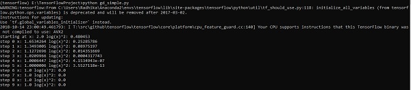
We can see that the necessary epochs and iterations are calculated as shown in the output.
我们可以看到,如输出所示,计算了必要的纪元和迭代。
TensorFlow-形成图 (TensorFlow - Forming Graphs)
A partial differential equation (PDE) is a differential equation, which involves partial derivatives with unknown function of several independent variables. With reference to partial differential equations, we will focus on creating new graphs.
偏微分方程(PDE)是一个微分方程,它涉及具有多个独立变量的未知函数的偏导数。 关于偏微分方程,我们将专注于创建新图。
Let us assume there is a pond with dimension 500*500 square −
让我们假设有一个尺寸为500 * 500平方的池塘-
N = 500
N = 500
Now, we will compute partial differential equation and form the respective graph using it. Consider the steps given below for computing graph.
现在,我们将计算偏微分方程并使用它形成相应的图。 考虑下面给出的计算图形的步骤。
Step 1 − Import libraries for simulation.
步骤1-导入库以进行仿真。
import tensorflow as tf
import numpy as np
import matplotlib.pyplot as plt
Step 2 − Include functions for transformation of a 2D array into a convolution kernel and simplified 2D convolution operation.
步骤2-包括用于将2D数组转换为卷积内核和简化2D卷积运算的函数。
def make_kernel(a):
   a = np.asarray(a)
   a = a.reshape(list(a.shape) + [1,1])
   return tf.constant(a, dtype=1)

def simple_conv(x, k):
   """A simplified 2D convolution operation"""
   x = tf.expand_dims(tf.expand_dims(x, 0), -1)
   y = tf.nn.depthwise_conv2d(x, k, [1, 1, 1, 1], padding = 'SAME')
   return y[0, :, :, 0]

def laplace(x):
   """Compute the 2D laplacian of an array"""
   laplace_k = make_kernel([[0.5, 1.0, 0.5], [1.0, -6., 1.0], [0.5, 1.0, 0.5]])
   return simple_conv(x, laplace_k)

sess = tf.InteractiveSession()
Step 3 − Include the number of iterations and compute the graph to display the records accordingly.
步骤3-包括迭代次数并计算图以相应地显示记录。
N = 500

# Initial Conditions -- some rain drops hit a pond

# Set everything to zero
u_init = np.zeros([N, N], dtype = np.float32)
ut_init = np.zeros([N, N], dtype = np.float32)

# Some rain drops hit a pond at random points
for n in range(100):
   a,b = np.random.randint(0, N, 2)
   u_init[a,b] = np.random.uniform()

plt.imshow(u_init)
plt.show()

# Parameters:
# eps -- time resolution
# damping -- wave damping
eps = tf.placeholder(tf.float32, shape = ())
damping = tf.placeholder(tf.float32, shape = ())

# Create variables for simulation state
U = tf.Variable(u_init)
Ut = tf.Variable(ut_init)

# Discretized PDE update rules
U_ = U + eps * Ut
Ut_ = Ut + eps * (laplace(U) - damping * Ut)

# Operation to update the state
step = tf.group(U.assign(U_), Ut.assign(Ut_))

# Initialize state to initial conditions
tf.initialize_all_variables().run()

# Run 1000 steps of PDE
for i in range(1000):
   # Step simulation
   step.run({eps: 0.03, damping: 0.04})

   # Visualize every 50 steps
   if i % 500 == 0:
      plt.imshow(U.eval())
      plt.show()
The graphs are plotted as shown below −
图形如下图所示-


使用TensorFlow进行图像识别 (Image Recognition using TensorFlow)
TensorFlow includes a special feature of image recognition and these images are stored in a specific folder. With relatively same images, it will be easy to implement this logic for security purposes.
TensorFlow包含图像识别的特殊功能,并且这些图像存储在特定的文件夹中。 对于相对相同的映像,出于安全目的很容易实现此逻辑。
The folder structure of image recognition code implementation is as shown below −
图像识别代码实现的文件夹结构如下图所示-

The dataset_image includes the related images, which need to be loaded. We will focus on image recognition with our logo defined in it. The images are loaded with “load_data.py” script, which helps in keeping a note on various image recognition modules within them.
dataset_image包括需要加载的相关图像。 我们将专注于其中定义了徽标的图像识别。 图像使用“ load_data.py”脚本加载,这有助于在其中的各个图像识别模块上保留注释。
import pickle
from sklearn.model_selection import train_test_split
from scipy import misc

import numpy as np
import os

label = os.listdir("dataset_image")
label = label[1:]
dataset = []

for image_label in label:
   images = os.listdir("dataset_image/"+image_label)

   for image in images:
      img = misc.imread("dataset_image/"+image_label+"/"+image)
      img = misc.imresize(img, (64, 64))
      dataset.append((img,image_label))
X = []
Y = []

for input,image_label in dataset:
   X.append(input)
   Y.append(label.index(image_label))

X = np.array(X)
Y = np.array(Y)

X_train,y_train, = X,Y

data_set = (X_train,y_train)

save_label = open("int_to_word_out.pickle","wb")
pickle.dump(label, save_label)
save_label.close()
The training of images helps in storing the recognizable patterns within specified folder.
图像训练有助于将可识别的图案存储在指定的文件夹中。
import numpy
import matplotlib.pyplot as plt

from keras.layers import Dropout
from keras.layers import Flatten
from keras.constraints import maxnorm
from keras.optimizers import SGD
from keras.layers import Conv2D
from keras.layers.convolutional import MaxPooling2D
from keras.utils import np_utils
from keras import backend as K

import load_data
from keras.models import Sequential
from keras.layers import Dense

import keras
K.set_image_dim_ordering('tf')

# fix random seed for reproducibility
seed = 7
numpy.random.seed(seed)

# load data
(X_train,y_train) = load_data.data_set

# normalize inputs from 0-255 to 0.0-1.0
X_train = X_train.astype('float32')

#X_test = X_test.astype('float32')
X_train = X_train / 255.0

#X_test = X_test / 255.0
# one hot encode outputs
y_train = np_utils.to_categorical(y_train)

#y_test = np_utils.to_categorical(y_test)
num_classes = y_train.shape[1]

# Create the model
model = Sequential()
model.add(Conv2D(32, (3, 3), input_shape = (64, 64, 3), padding = 'same',
   activation = 'relu', kernel_constraint = maxnorm(3)))

model.add(Dropout(0.2))
model.add(Conv2D(32, (3, 3), activation = 'relu', padding = 'same',
   kernel_constraint = maxnorm(3)))

model.add(MaxPooling2D(pool_size = (2, 2)))
model.add(Flatten())
model.add(Dense(512, activation = 'relu', kernel_constraint = maxnorm(3)))
model.add(Dropout(0.5))
model.add(Dense(num_classes, activation = 'softmax'))

# Compile model
epochs = 10
lrate = 0.01
decay = lrate/epochs
sgd = SGD(lr = lrate, momentum = 0.9, decay = decay, nesterov = False)
model.compile(loss = 'categorical_crossentropy', optimizer = sgd, metrics = ['accuracy'])
print(model.summary())

#callbacks = [keras.callbacks.EarlyStopping(
   monitor = 'val_loss', min_delta = 0, patience = 0, verbose = 0, mode = 'auto')]
callbacks = [keras.callbacks.TensorBoard(log_dir='./logs',
   histogram_freq = 0, batch_size = 32, write_graph = True, write_grads = False,
   write_images = True, embeddings_freq = 0, embeddings_layer_names = None,
   embeddings_metadata = None)]

# Fit the model

model.fit(X_train, y_train, epochs = epochs,
   batch_size = 32,shuffle = True,callbacks = callbacks)

# Final evaluation of the model
scores = model.evaluate(X_train, y_train, verbose = 0)
print("Accuracy: %.2f%%" % (scores[1]*100))

# serialize model to JSONx
model_json = model.to_json()
with open("model_face.json", "w") as json_file:
   json_file.write(model_json)

# serialize weights to HDF5
model.save_weights("model_face.h5")
print("Saved model to disk")
The above line of code generates an output as shown below −
上面的代码行生成如下所示的输出-


神经网络培训建议 (Recommendations for Neural Network Training)
In this chapter, we will understand the various aspects of neural network training which can be implemented using TensorFlow framework.
在本章中,我们将了解可以使用TensorFlow框架实现的神经网络训练的各个方面。
Following are the ten recommendations, which can be evaluated −
以下是十项建议,可以对其进行评估-
反向传播 (Back Propagation)
Back propagation is a simple method to compute partial derivatives, which includes the basic form of composition best suitable for neural nets.
反向传播是一种计算偏导数的简单方法,其中包括最适合神经网络的基本组成形式。

随机梯度下降 (Stochastic Gradient Descent)
In stochastic gradient descent, a batch is the total number of examples, which a user uses to calculate the gradient in a single iteration. So far, it is assumed that the batch has been the entire data set. The best illustration is working at Google scale; data sets often contain billions or even hundreds of billions of examples.
在随机梯度下降中, 批处理是示例总数,用户可使用该示例在一次迭代中计算梯度。 到目前为止,假定批处理已成为整个数据集。 最好的例证是在Google规模上工作。 数据集通常包含数十亿甚至数千亿个示例。

学习率衰减 (Learning Rate Decay)

Adapting the learning rate is one of the most important features of gradient descent optimization. This is crucial to TensorFlow implementation.
适应学习率是梯度下降优化的最重要特征之一。 这对于TensorFlow实施至关重要。
退出 (Dropout)
Deep neural nets with a large number of parameters form powerful machine learning systems. However, over fitting is a serious problem in such networks.
具有大量参数的深度神经网络形成了功能强大的机器学习系统。 但是,在这种网络中,过度拟合是一个严重的问题。

最大池 (Max Pooling)
Max pooling is a sample-based discretization process. The object is to down-sample an input representation, which reduces the dimensionality with the required assumptions.
最大池化是基于样本的离散化过程。 目的是对输入表示进行下采样,以减少所需假设的维数。

长短期记忆(LSTM) (Long Short Term Memory (LSTM))
LSTM controls the decision on what inputs should be taken within the specified neuron. It includes the control on deciding what should be computed and what output should be generated.
LSTM控制在指定神经元内应采取哪些输入的决策。 它包括决定应该计算什么和应该产生什么输出的控制。

翻译自: https://www.tutorialspoint.com/tensorflow/tensorflow_quick_guide.htm


 4097
4097

 被折叠的 条评论
为什么被折叠?
被折叠的 条评论
为什么被折叠?
 到【灌水乐园】发言


