Python利用pandas/sklearn处理类别型特征；手动分段与离散化处理连续型特征

类别型变量特征：

独热向量编码/One-Hot-Encoding (Dummy variables)
颜色：红、黄、紫[1,0,0] [0,1,0] [0,0,1] LR = theta*X
红色 蓝色 黄色 紫色 咖啡色 白色… => 红色 蓝色 黄色 rare
sklearn OneHotEncoder；pandas get_dummies

# create a dataframe with an integer feature and a categorical string feature
import pandas as pd
demo_df = pd.DataFrame({'Integer Feature': [0, 1, 2, 1], 'Categorical Feature': ['socks', 'fox', 'socks', 'box']})
demo_df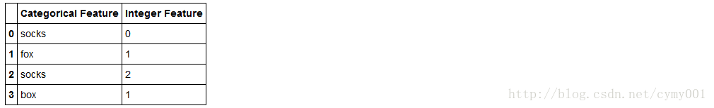

pd.get_dummies(demo_df)   #get_dummies对“整数特征”无变化，对“类别特征”one-hot编码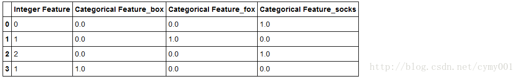

demo_df['Integer Feature'] = demo_df['Integer Feature'].astype(str)
pd.get_dummies(demo_df)   #将“整数特征”变成“字符型类别”进行one-hot编码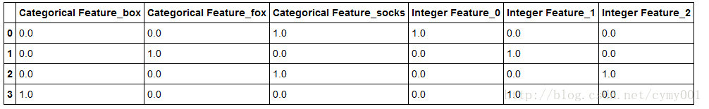

连续型变量特征：

连续数据分桶，拿到数据对应桶编号，分桶边界可以自己基于统计给出

地铁上让座的问题
年龄：0-100
LR？theta确定，要么就是和x成正相关，要么就是和x成负相关
0-100
[0-6](6-10](10,30](30,50](50…
[1,0,0,0,0,…]
[0,1,…]

#mglearn包里的make_wave函数
import numpy as np
def make_wave(n_samples=100):
    rnd = np.random.RandomState(42)
    x = rnd.uniform(-3, 3, size=n_samples)   #np.random.uniform生成100个随机数,符合U(-3,3)上的均匀分布
    y_no_noise = (np.sin(4 * x) + x)
    y = (y_no_noise + rnd.normal(size=len(x))) / 2   np.random.normal
    #生成100个随机数,符合N(0,1)正态分布
    return x.reshape(-1, 1), y   #返回关于x的列向量

%matplotlib inline
from preamble import *
from sklearn.linear_model import LinearRegression
from sklearn.tree import DecisionTreeRegressor
X, y = mglearn.datasets.make_wave(n_samples=100)   
#利用mglearn包里的函数制作数据集
plt.plot(X[:, 0], y, 'o')
line = np.linspace(-3, 3, 1000)[:-1].reshape(-1, 1)   #列向量
reg = LinearRegression().fit(X, y)
plt.plot(line, reg.predict(line), label="linear regression")
reg = DecisionTreeRegressor(min_samples_split=3).fit(X, y)   #min_samples_split参数指定树内点分裂至少要有3个样本点
plt.plot(line, reg.predict(line), label="decision tree")
plt.ylabel("regression output")
plt.xlabel("input feature")
plt.legend(loc="best")

import numpy as np
np.set_printoptions(precision=2)   
#np.set_printoptions设置数组打印信息，precision设置输出浮点数精度
bins = np.linspace(-3, 3, 11)   #构造连续特征切割分桶边界
bins
#Output:
#array([-3. , -2.4, -1.8, -1.2, -0.6,  0. ,  0.6,  1.2,  1.8,  2.4,  3. ])

which_bin = np.digitize(X, bins=bins)    #np.digitize返回参数数组对应分桶的索引
print("\nData points:\n", X[:5])
print("\nBin membership for data points:\n", which_bin[:5])
#Output:
#Data points:
# [[-0.75]
# [ 2.7 ]
# [ 1.39]
# [ 0.59]
# [-2.06]]
#Bin membership for data points:
# [[ 4]
# [10]
# [ 8]
# [ 6]
# [ 2]]

from sklearn.preprocessing import OneHotEncoder
# transform using the OneHotEncoder.
encoder = OneHotEncoder(sparse=False)   #sparse参数设置为True,使输出为系数矩阵形式；否则为数组
# encoder.fit finds the unique values that appear in which_bin
encoder.fit(which_bin)   #根据索引数组,one-hot成稀疏矩阵
# transform creates the one-hot encoding
X_binned = encoder.transform(which_bin)   #X_binned是one-hot变换后的训练数据集
print(X_binned[:5])
#Output:
#[[ 0.  0.  0.  1.  0.  0.  0.  0.  0.  0.]
# [ 0.  0.  0.  0.  0.  0.  0.  0.  0.  1.]
# [ 0.  0.  0.  0.  0.  0.  0.  1.  0.  0.]
# [ 0.  0.  0.  0.  0.  1.  0.  0.  0.  0.]
# [ 0.  1.  0.  0.  0.  0.  0.  0.  0.  0.]]

X_binned.shape
#Output:
#(100,10)

line_binned = encoder.transform(np.digitize(line, bins=bins))   #line_binned是one-hot变换后的测试数据集

plt.plot(X[:, 0], y, 'o')
reg = LinearRegression().fit(X_binned, y)   
plt.plot(line, reg.predict(line_binned), label='linear regression binned')   

reg = DecisionTreeRegressor(min_samples_split=3).fit(X_binned, y)
plt.plot(line, reg.predict(line_binned), linewidth=2.5, linestyle='-.', label='decision tree binned')
for bin in bins:
    plt.plot([bin, bin], [-3, 3], ':', c='k')   #分段考虑,线性回归
plt.legend(loc="best")
plt.suptitle("linear_binning")