吴恩达机器学习作业——正则化线性回归及偏差和方差

自变量x——水库中水量变化；因变量y——水坝外水流量。

任务：1.预测 2.诊断算法错误。

训练集：X,y 

交叉集：Xval,yval

测试集：Xtest,ytest

1显示图像

fprintf('Loading and Visualizing Data ...\n')
load ('ex5data1.mat');
m = size(X, 1);
plot(X, y, 'rx', 'MarkerSize', 10, 'LineWidth', 1.5);
xlabel('Change in water level (x)');
ylabel('Water flowing out of the dam (y)');

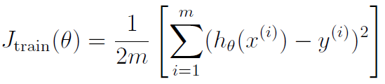
2正则化线性回归代价函数和梯度

theta = [1 ; 1];
J = linearRegCostFunction([ones(m, 1) X], y, theta, 1);

fprintf(['Cost at theta = [1 ; 1]: %f '...
         '\n(this value should be about 303.993192)\n'], J);

theta = [1 ; 1];
[J, grad] = linearRegCostFunction([ones(m, 1) X], y, theta, 1);

fprintf(['Gradient at theta = [1 ; 1]:  [%f; %f] '...
         '\n(this value should be about [-15.303016; 598.250744])\n'], ...
         grad(1), grad(2));

linearRegCostFunction函数如下：

function [J, grad] = linearRegCostFunction(X, y, theta, lambda)
m = length(y);
J = 0;
grad = zeros(size(theta));
J = (sum(((X*theta)-y).^2))/(2*m)+(lambda/(2*m))*(sum(theta.^2)-theta(1)^2);
grad = (1/m)*X'*(X*theta-y)+[0;(lambda/m)*theta(2:end)];
grad = grad(:);
end
%正则化不考虑第一个theta。

3训练线性回归

fmincg用来求解训练集中使得J最小的theta，求解出的theta用来做线性回归（但实际数据为非线性，然后再诊断错误。）

% 绘制线性图
lambda = 0;
[theta] = trainLinearReg([ones(m, 1) X], y, lambda);
plot(X, y, 'rx', 'MarkerSize', 10, 'LineWidth', 1.5);
xlabel('Change in water level (x)');
ylabel('Water flowing out of the dam (y)');
hold on;
plot(X, [ones(m, 1) X]*theta, '--', 'LineWidth', 2) %画直线，增加一列值为1的x，变为y=kx+b形式。
hold off;

trainLinearReg函数：

function [theta] = trainLinearReg(X, y, lambda)
initial_theta = zeros(size(X, 2), 1); %初始化theta
costFunction = @(t) linearRegCostFunction(X, y, t, lambda); %前面计算的代价函数
options = optimset('MaxIter', 200, 'GradObj', 'on'); %最大迭代次数
theta = fmincg(costFunction, initial_theta, options); %fmincg函数求解最优theta
end

fmincg函数（不必完全掌握）：

function [X, fX, i] = fmincg(f, X, options, P1, P2, P3, P4, P5)
if exist('options', 'var') && ~isempty(options) && isfield(options, 'MaxIter')
    length = options.MaxIter;
else
    length = 100;
end


RHO = 0.01;                            % a bunch of constants for line searches
SIG = 0.5;       % RHO and SIG are the constants in the Wolfe-Powell conditions
INT = 0.1;    % don't reevaluate within 0.1 of the limit of the current bracket
EXT = 3.0;                    % extrapolate maximum 3 times the current bracket
MAX = 20;                         % max 20 function evaluations per line search
RATIO = 100;                                      % maximum allowed slope ratio

argstr = ['feval(f, X'];                      % compose string used to call function
for i = 1:(nargin - 3)
  argstr = [argstr, ',P', int2str(i)];
end
argstr = [argstr, ')'];

if max(size(length)) == 2, red=length(2); length=length(1); else red=1; end
S=['Iteration '];

i = 0;                                            % zero the run length counter
ls_failed = 0;                             % no previous line search has failed
fX = [];
[f1 df1] = eval(argstr);                      % get function value and gradient
i = i + (length<0);                                            % count epochs?!
s = -df1;                                        % search direction is steepest
d1 = -s'*s;                                                 % this is the slope
z1 = red/(1-d1);                                  % initial step is red/(|s|+1)

while i < abs(length)                                      % while not finished
  i = i + (length>0);                                      % count iterations?!

  X0 = X; f0 = f1; df0 = df1;                   % make a copy of current values
  X = X + z1*s;                                             % begin line search
  [f2 df2] = eval(argstr);
  i = i + (length<0);                                          % count epochs?!
  d2 = df2'*s;
  f3 = f1; d3 = d1; z3 = -z1;             % initialize point 3 equal to point 1
  if length>0, M = MAX; else M = min(MAX, -length-i); end
  success = 0; limit = -1;                     % initialize quanteties
  while 1
    while ((f2 > f1+z1*RHO*d1) || (d2 > -SIG*d1)) && (M > 0) 
      limit = z1;                                         % tighten the bracket
      if f2 > f1
        z2 = z3 - (0.5*d3*z3*z3)/(d3*z3+f2-f3);                 % quadratic fit
      else
        A = 6*(f2-f3)/z3+3*(d2+d3);                                 % cubic fit
        B = 3*(f3-f2)-z3*(d3+2*d2);
        z2 = (sqrt(B*B-A*d2*z3*z3)-B)/A;       % numerical error possible - ok!
      end
      if isnan(z2) || isinf(z2)
        z2 = z3/2;                  % if we had a numerical problem then bisect
      end
      z2 = max(min(z2, INT*z3),(1-INT)*z3);  % don't accept too close to limits
      z1 = z1 + z2;                                           % update the step
      X = X + z2*s;
      [f2 df2] = eval(argstr);
      M = M - 1; i = i + (length<0);                           % count epochs?!
      d2 = df2'*s;
      z3 = z3-z2;                    % z3 is now relative to the location of z2
    end
    if f2 > f1+z1*RHO*d1 || d2 > -SIG*d1
      break;                                                % this is a failure
    elseif d2 > SIG*d1
      success = 1; break;                                             % success
    elseif M == 0
      break;                                                          % failure
    end
    A = 6*(f2-f3)/z3+3*(d2+d3);                      % make cubic extrapolation
    B = 3*(f3-f2)-z3*(d3+2*d2);
    z2 = -d2*z3*z3/(B+sqrt(B*B-A*d2*z3*z3));        % num. error possible - ok!
    if ~isreal(z2) || isnan(z2) || isinf(z2) || z2 < 0 % num prob or wrong sign?
      if limit < -0.5                               % if we have no upper limit
        z2 = z1 * (EXT-1);                 % the extrapolate the maximum amount
      else
        z2 = (limit-z1)/2;                                   % otherwise bisect
      end
    elseif (limit > -0.5) && (z2+z1 > limit)         % extraplation beyond max?
      z2 = (limit-z1)/2;                                               % bisect
    elseif (limit < -0.5) && (z2+z1 > z1*EXT)       % extrapolation beyond limit
      z2 = z1*(EXT-1.0);                           % set to extrapolation limit
    elseif z2 < -z3*INT
      z2 = -z3*INT;
    elseif (limit > -0.5) && (z2 < (limit-z1)*(1.0-INT))  % too close to limit?
      z2 = (limit-z1)*(1.0-INT);
    end
    f3 = f2; d3 = d2; z3 = -z2;                  % set point 3 equal to point 2
    z1 = z1 + z2; X = X + z2*s;                      % update current estimates
    [f2 df2] = eval(argstr);
    M = M - 1; i = i + (length<0);                             % count epochs?!
    d2 = df2'*s;
  end                                                      % end of line search

  if success                                         % if line search succeeded
    f1 = f2; fX = [fX' f1]';
    fprintf('%s %4i | Cost: %4.6e\r', S, i, f1);
    s = (df2'*df2-df1'*df2)/(df1'*df1)*s - df2;      % Polack-Ribiere direction
    tmp = df1; df1 = df2; df2 = tmp;                         % swap derivatives
    d2 = df1'*s;
    if d2 > 0                                      % new slope must be negative
      s = -df1;                              % otherwise use steepest direction
      d2 = -s'*s;    
    end
    z1 = z1 * min(RATIO, d1/(d2-realmin));          % slope ratio but max RATIO
    d1 = d2;
    ls_failed = 0;                              % this line search did not fail
  else
    X = X0; f1 = f0; df1 = df0;  % restore point from before failed line search
    if ls_failed || i > abs(length)          % line search failed twice in a row
      break;                             % or we ran out of time, so we give up
    end
    tmp = df1; df1 = df2; df2 = tmp;                         % swap derivatives
    s = -df1;                                                    % try steepest
    d1 = -s'*s;
    z1 = 1/(1-d1);                     
    ls_failed = 1;                                    % this line search failed
  end
  if exist('OCTAVE_VERSION')
    fflush(stdout);
  end
end
fprintf('\n');

结果：

4线性回归的学习曲线

绘制学习曲线：

lambda = 0;
[error_train, error_val] = ...
    learningCurve([ones(m, 1) X], y, ...
                  [ones(size(Xval, 1), 1) Xval], yval, ...
                  lambda);

plot(1:m, error_train, 1:m, error_val);
title('Learning curve for linear regression')
legend('Train', 'Cross Validation')
xlabel('Number of training examples')
ylabel('Error')
axis([0 13 0 150])

fprintf('# Training Examples\tTrain Error\tCross Validation Error\n');
for i = 1:m
    fprintf('  \t%d\t\t%f\t%f\n', i, error_train(i), error_val(i));
end

此时检验误差的函数为（若为交叉集，替换为交叉集的X,y，m替换为交叉集的数量），没有lambda：

learningCurve函数：

function [error_train, error_val] = ...
    learningCurve(X, y, Xval, yval, lambda)
m = size(X, 1);

error_train = zeros(m, 1);
error_val   = zeros(m, 1);
for i=1:m
    theta = trainLinearReg(X(1:i, :), y(1:i), lambda);
    error_train(i) = linearRegCostFunction(X(1:i, :), y(1:i), theta, 0);
    error_val(i) = linearRegCostFunction(Xval, yval, theta, 0);
end

学习曲线图如下：

理解：因为theta是根据训练集得出的，且欠拟合。所以蓝色线样本数少的时候误差很小，样本数量多时误差增大；但红色线，即交叉集，是未知数据，因此数据少时误差很大，随着样本数据增加误差慢慢接近训练集误差。因此，再增加样本数量结果仍然如此，所以增加样本数量对于欠拟合模型是无用的。接下来增加自变量的指数来解决欠拟合问题。

5多项式回归的特征映射

首先，定义指数为8次幂。

将X,Xval和Xtest的每一列变为X的n次幂（1~8次幂）结果，代码如下：

p = 8;
X_poly = polyFeatures(X, p);
[X_poly, mu, sigma] = featureNormalize(X_poly);  % Normalize归一化，解决特征取值范围过大问题。
X_poly = [ones(m, 1), X_poly];                   % Add Ones

% Map X_poly_test and normalize (using mu and sigma)
X_poly_test = polyFeatures(Xtest, p);
X_poly_test = bsxfun(@minus, X_poly_test, mu);
X_poly_test = bsxfun(@rdivide, X_poly_test, sigma);
X_poly_test = [ones(size(X_poly_test, 1), 1), X_poly_test];         % Add Ones

% Map X_poly_val and normalize (using mu and sigma)
X_poly_val = polyFeatures(Xval, p);
X_poly_val = bsxfun(@minus, X_poly_val, mu);
X_poly_val = bsxfun(@rdivide, X_poly_val, sigma);
X_poly_val = [ones(size(X_poly_val, 1), 1), X_poly_val];           % Add Ones

fprintf('Normalized Training Example 1:\n');
fprintf('  %f  \n', X_poly(1, :));

ployFeatures函数将X变为次幂矩阵：

function [X_poly] = polyFeatures(X, p)
X_poly = zeros(numel(X), p);
X_poly = [X X.^2 X.^3 X.^4 X.^5 X.^6 X.^7 X.^8]; 
%也可用循环
%for i = 1:p
%X_poly(:,i) = X.^i;
%end
end

归一化函数featureNormalize：

function [X_norm, mu, sigma] = featureNormalize(X)
mu = mean(X);
X_norm = bsxfun(@minus, X, mu);
sigma = std(X_norm);
X_norm = bsxfun(@rdivide, X_norm, sigma);
end

最终以X为例，增加指数并归一化后的矩阵为：

6为多项式回归绘制学习曲线

首先，绘制拟合曲线。

lambda = 0;
[theta] = trainLinearReg(X_poly, y, lambda);%利用训练集优化出的theta
figure(1);
plot(X, y, 'rx', 'MarkerSize', 10, 'LineWidth', 1.5);
plotFit(min(X), max(X), mu, sigma, theta, p);
xlabel('Change in water level (x)');
ylabel('Water flowing out of the dam (y)');
title (sprintf('Polynomial Regression Fit (lambda = %f)', lambda));

其中 plot函数画点，plotFit函数画线。

function plotFit(min_x, max_x, mu, sigma, theta, p)
hold on;
x = (min_x - 15: 0.05 : max_x + 25)';%看一下已知数据范围外的变化。
X_poly = polyFeatures(x, p);
X_poly = bsxfun(@minus, X_poly, mu);
X_poly = bsxfun(@rdivide, X_poly, sigma);
X_poly = [ones(size(x, 1), 1) X_poly];
plot(x, X_poly * theta, '--', 'LineWidth', 2)
hold off
end

曲线如下：

绘制学习曲线：

figure(2);
[error_train, error_val] = ...
    learningCurve(X_poly, y, X_poly_val, yval, lambda);
plot(1:m, error_train, 1:m, error_val);

title(sprintf('Polynomial Regression Learning Curve (lambda = %f)', lambda));
xlabel('Number of training examples')
ylabel('Error')
axis([0 13 0 100]) %横坐标为0~13，纵坐标为0~100
legend('Train', 'Cross Validation')

fprintf('Polynomial Regression (lambda = %f)\n\n', lambda);
fprintf('# Training Examples\tTrain Error\tCross Validation Error\n');
for i = 1:m
    fprintf('  \t%d\t\t%f\t%f\n', i, error_train(i), error_val(i));
end

曲线如下（下面又一条蓝线为训练集误差，值基本为0）：

从左到右依次是：样本数，训练集误差，交叉集误差。（上图的自变量和因变量）

上述结果可能过拟合，因此下面练习利用不同的正则化参数lambda来纠正过拟合。

7为选择的λ参数进行验证

（1）若选择的λ=1，拟合曲线和学习曲线分别为（λ过小）

（2）若选择的λ=100，拟合曲线和学习曲线分别为（λ过大）

合适的λ需要学习曲线中训练集和交叉验证集的误差都很小且接近。

自动选择最佳λ的方法：以lambda为横坐标，误差为纵坐标绘制曲线。选取交叉验证集中误差最小的λ作为最佳值。

[lambda_vec, error_train, error_val] = ...
    validationCurve(X_poly, y, X_poly_val, yval);

close all;
plot(lambda_vec, error_train, lambda_vec, error_val);%以lambda为横坐标，误差为纵坐标绘制曲线。
legend('Train', 'Cross Validation');
xlabel('lambda');
ylabel('Error');
axis([0 10 0 20])

fprintf('lambda\t\tTrain Error\tValidation Error\n');
for i = 1:length(lambda_vec)
	fprintf(' %f\t%f\t%f\n', ...
            lambda_vec(i), error_train(i), error_val(i));
end

其中，λ取值实验：lambda_vec = [0 0.001 0.003 0.01 0.03 0.1 0.3 1 3 10]';

function [lambda_vec, error_train, error_val] = ...
    validationCurve(X, y, Xval, yval)
lambda_vec = [0 0.001 0.003 0.01 0.03 0.1 0.3 1 3 10]';
error_train = zeros(length(lambda_vec), 1);
error_val = zeros(length(lambda_vec), 1);
for i=1:length(lambda_vec)
    theta = trainLinearReg(X, y, lambda_vec(i));
    error_train(i) = linearRegCostFunction(X, y, theta, 0);
    error_val(i) = linearRegCostFunction(Xval, yval, theta, 0);
end

绘制出的曲线为（lambda约为3）

此时的拟合曲线以及学习曲线为（训练集和交叉集误差很小且接近）：