【R语言】绘制带中国轮廓及九段线的渲染地图

一、中国轮廓和九段线分别添加

1.用到的R包

library(sf)
library(ggspatial)
library(ggplot2)
library(cowplot)
library(colorspace)

2.输入数据

# 读入中国区县分布数据
china <- sf::read_sf('./地图文件geojson/中国省级地图GS（2019）1719号.geojson')
# 读入九段线数据
nine_lines <- sf::read_sf('./地图文件geojson/九段线GS（2019）1719号.geojson')
station_shp  <- st_read("./plot70.shp")   #渲染的数据shp文件，比如各省市的人口密度
#用st_read读取的shp不会出现中文乱码

3.绘图

L <- 10
barwidth <- 8
barheight <-  0.5
breakc =c(-L,-L/2,0,L/2,L)
labelc =c(paste0('≤',-L),-L/2,0,L/2,paste0('≥',L))
title = "title)"  #标题自己命名
col1 = colorRampPalette(c("#C82423","#db6968","#F8AC8C",'#FFF
                          '#87CEFA',"#1E90FF","#0074b3"))(41)
 #绘制中国地图
p=ggplot() +
  geom_sf(data=china, fill= "NA", size=0.6, color='grey') + # 中国地图轮廓
  geom_sf(data=station_shp,aes(fill=trendobs))+
  scale_fill_gradientn(colours = col1,  na.value = 'transparent',
                       breaks=breakc,labels=labelc  )+
  coord_sf(ylim = c(-2387082,1654989), crs='+proj=laea +lat_0=40 +lon_0=104') + #截取中国地图，不在大图上显示九段线区域，这个范围不要改
  guides(fill = guide_colorbar(barwidth = barwidth, barheight = barheight, 
                               title=title ),
         title.position = "top")+
  annotate('text', x = -Inf, y = Inf, label = 'Obs', 
           hjust = -0.5, vjust = 2, fontface = 'bold', size = 4)+
  theme(rect=element_blank(),
        panel.background=element_blank(),
        panel.grid=element_blank(),
        axis.line=element_blank(),
        axis.text=element_blank(),
        axis.ticks=element_blank(),
        axis.title = element_blank(),
        legend.key.size = unit(10, "pt"),
        legend.title= element_text(size=10),
        legend.position = "bottom" ,
        legend.box = "horizontal")
# 绘制九段线小图
nine_map = ggplot() +
  geom_sf(data = china,fill='NA', size=0.5) + 
  geom_sf(data = nine_lines,color='black',size=0.5)+
  coord_sf(ylim = c(-4028017,-1877844),xlim = c(117131.4,2115095),crs="+proj=laea +lat_0=40 +lon_0=104")+
  theme(
    aspect.ratio = 1.25, #调节长宽比
    axis.text = element_blank(),
    axis.ticks = element_blank(),
    axis.title = element_blank(),
    panel.grid = element_blank(),
    panel.background = element_blank(),
    panel.border = element_rect(fill=NA,color="grey10",linetype=1,size=0.5),
    plot.margin=unit(c(0,0,0,0),"mm"))
# 使用cowplot包将大图小图拼在一起
fig = ggdraw() +
  draw_plot(p) +
  draw_plot(nine_map, x = 0.79, y = 0.15, width = 0.13, height = 0.39)
#出图
png('./seslut/fig.png',width = 6, height =9, res = 500, units = 'in')
plot(fig)
dev.off()                   

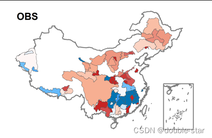
4.成图效果，仅作展示

二、中国轮廓和九段线合并为一个shp时

2.数据输入

china <- sf::st_read('./map/国界new.shp')  #合并后的shp
station_shp  <- st_read("./plot70.shp")   #渲染的数据shp文件，比如各省市的人口密度
#用st_read读取的shp不会出现中文乱码

3.绘图

L <- 10
barwidth <- 8
barheight <-  0.5
breakc =c(-L,-L/2,0,L/2,L)
labelc =c(paste0('≤',-L),-L/2,0,L/2,paste0('≥',L))
title = "title)"  #标题自己命名
col1 = colorRampPalette(c("#C82423","#db6968","#F8AC8C",'#FFF
                          '#87CEFA',"#1E90FF","#0074b3"))(41)

p=ggplot() +
  geom_sf(data=china, fill= "NA", size=0.6
  geom_sf(data=station_shp,aes(fill=trendo
  scale_fill_gradientn(colours = col1,  na
                       breaks=breakc,label

  guides(fill = guide_colorbar(barwidth = 
                               title=title
         title.position = "top")+
  annotate('text', x = -Inf, y = Inf, labe
           hjust = -0.5, vjust = 2, fontfa
  theme(rect=element_blank(),
        panel.background=element_blank(),
        panel.grid=element_blank(),
        axis.line=element_blank(),
        axis.text=element_blank(),
        axis.ticks=element_blank(),
        axis.title = element_blank(),
        legend.key.size = unit(10, "pt"),
        legend.title= element_text(size=10
        legend.position = "none" ,
        legend.box = "horizontal")
#其他代码一致

4.出图效果，同上