Large scale machine learning - Stochastic gradient descent convergence

In this class, let's talk about:

1. How to make sure the Stochastic gradient descent algorithm is converging well when we're running the algorithm
2. How to tune the learning rate for the algorithm.

figure-1

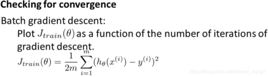
As what can be seen in figure-1, when we were using batch gradient descent, our standard way for making sure that gradient descent was converging was we would plot the optimization cost function () as a function of the number of iterations. And we would make sure that the cost function was decreasing on every iteration. When the training set was small, we could do that because we could compute the sum pretty efficiently. But when you have a massive training set size (e.g., 300 million), then you don't want to have to pause your algorithm periodically in order to compute this cost function.

figure-2

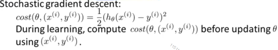
So for Stochastic gradient descent, in order to check the algorithm is converging, the figure-2 shows what we can do instead.

1. Right before we train on a specific example, that is before updating using , let's compute the cost of that example
2. Then, to check for the convergence of Stochastic gradient descent, every 1000 iterations (say), we can plot the cost averaged over the last 1000 examples. This can kind of give you a running estimate of how well the algorithm is doing. And let us check whether the algorithm is converging.

figure-3

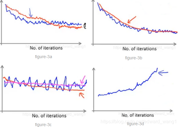
Some examples are shown in figure-3. Suppose you've plotted the cost average over the last 1000 examples.

• Because they are averaged over just 1000 examples, they're going to be a little bit noisy, so they may not decrease on every single iteration. Then if you get a figure looks like figure-3a, that would be a pretty decent run with the algorithm. It looks like the cost has gone down and then plateaued from specific point. Then maybe your learning algorithm has converged. If you want to try a smaller learning rate , something you might see is what shown by the red line. The algorithm may initially learn more slowly so the cost goes down more slowly. But then eventually with a smaller learning rate, it's actually possible for the algorithm to end up at a maybe very slightly better solution. The reason is that Stochastic gradient descent doesn't actually converge to the global minimum, instead the parameters will oscillate around the global minimum. By using a smaller learning rate, you'll end up with smaller oscillations.
• If instead averaging over 5000 examples, it's possible that you might get a smoother curve that looks like the red line in figure-3b. And so that's the effect of increasing the number of examples you average over. The disadvantage of making this too big is that now you get one data point only every 5000 examples. And so the feedback on how well your algorithm is doing is sort of delayed.
• Sometimes you may end up with a plot like the blue line in figure-3c. It looks like the cost not decreasing at all and thus the algorithm is not converging. But again if you were to average over a larger (say 5000) examples, it's possible that you see something like the red line. And it looks like the cost is actually decreasing. The blue line is too noisy and you couldnt' see the actual trend. Of course, it's also possible that the cost is still flat, as the magent line, even if you average over larger examples. If that is true, then it means the algorithm is not learning much for whatever reason. And you need either change the learning rate or change the features or change something else about the algorithm.
• Finally if you see a curve that is increasing as figure-3d, then this is a sign that the algorithm is diverging. What you usually do is use a smaller learning rate

Next, let's examine the issue of learning rate a little bit more.

figure-4

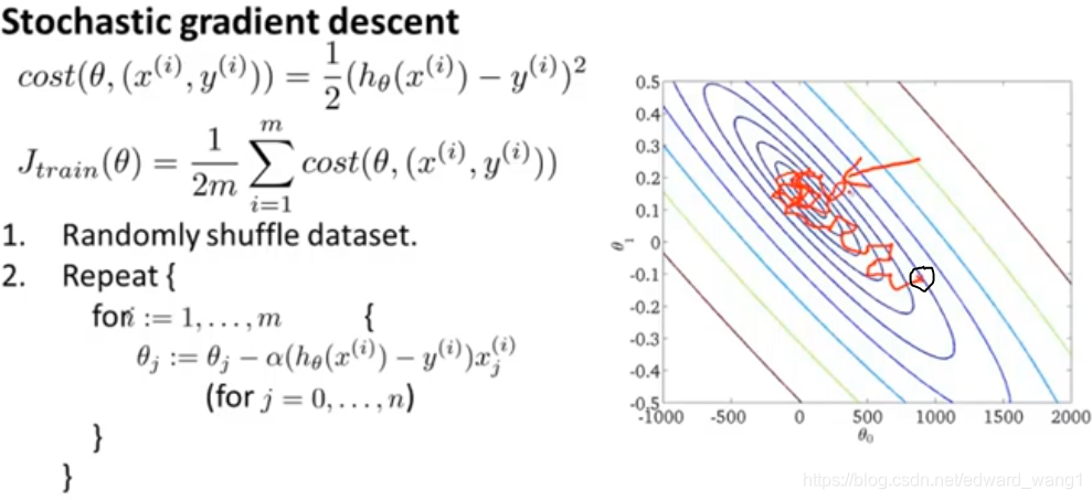
In figure-4, it's a review of Stochastic gradient algorithm. When you run the algorithm, it will start from some point and sort of meander towards the minimum. It won't really converge and instead it'll wander around the minimum forever. So you end up with a parameter value that is hopefully close to the global minimum that won't be exactly at the global minimum. In most typical applications of Stochastic gradient descent, the learning rate is typically held constant. So you typically will end up with a picture like figure-4.

If you want Stochastic gradient descent actually to converge to the global minimum, one thing you can do is slowly decrease the learning rate over time. A typical way for this is to define the learning rate as the following:

figure-5

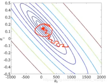
Where iterationNumber is really the number of training examples that have been scaned by Stochastic gradient descent algorithm. const1 and const2 are additional parameters that you might have to fiddle with a bit in order to get good performance. And if you manage to tune the parameters well, then the picture you can get would be as figure-5. At the beginning, the algorithm will actually meander around toward the minimum. But as it gets closer, because you're decreasing the learning rate, the meanderings will get smaller and smaller until it pretty much just converges to the global minimum.

In practice, people tend not to do this because you'll end up needing to spend time playing with these 2 extra parameters. This makes the algorithm more finicky. And frankly usually we're pretty happy with any parameter value that is pretty close to the  global minimum.

<end>