【Python】流程图神器PygraphViz详解

最近在做新的课程《风控策略自动化挖掘》，过程中要用到流程图，发现一个很好用的库pygraphviz，非常好用，我也只是探索了部分功能，这里分享给大家。

一、导入模块

import pygraphviz as pgv

二、创建图形

G = pgv.AGraph(directed=True, strict=False, nodesep=0, 
ranksep=1.2, rankdir="TB",               
splines="none", concentrate=True, bgcolor="write",               
compound=True, normalize=False, encoding='UTF-8'
)

参数解释

• directed -> False | True：有向图

• strict -> True | False：简单图

• nodesep：同级节点最小间距

• ranksep：不同级节点最小间距

• rankdir：绘图方向，可选 TB (从上到下), LR (从左到右), BT (从下到上), RL (从右到左)

• splines：线条类型，可选 ortho (直角), polyline (折线), spline (曲线), line (线条), none (无)

• concentrate -> True | False：合并线条 (双向箭头)

• bgcolor：背景颜色

• compound -> True | False：多子图时，不允许子图相互覆盖

• normalize -> False | True：以第一个节点作为顶节点

三、添加节点

G.add_node(name, label=None, fontname="Times-Roman", fontsize=14,
           shape="ellipse", style="rounded", color="black", fontcolor="black",
           pos="x,y(!)", fixedsize=False, width=1, height=1)
G.add_nodes_from(names, **attr) # 批量添加点，参数同上

参数解释

• name -> str：节点名。label 为节点标签，未指定时显示 name

• fontname：字体名称，常用：Microsoft YaHei, SimHei, KaiTi, SimSun, FangSong, Times-Roman, Helvetica, Courier。可以使用 "times bold italic" 表示字体类型、粗细、倾斜

• fixedsize -> Flase | True | "shape"`：固定大小，默认随文本长度变化。设置为 True 时，width 和 height 参数共同控制点大小。设置为 "shape" 时，将取标签文本和设置值的较大者

• style：节点线样式，使用 `color` 设置线条颜色 (style="filled" 时，设置填充颜色)

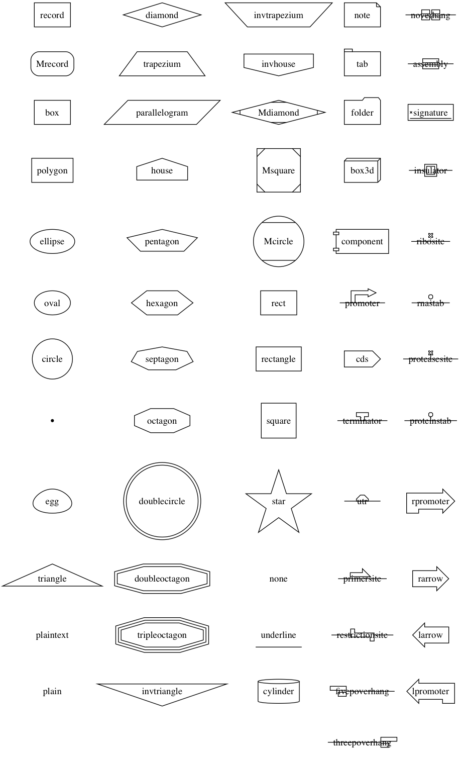
• shape：节点形状

• pos -> str：点的初始位置。使用 "x,y!" 时，可以强制固定点的位置。

四、 添加边

G.add_edge(origin, target, color="black", style="solid", 
penwidth=1,           
label="", fontname="Times-Roman", fontsize=14, 
fontcolor="black",           
arrowsize=1, arrowhead="normal", arrowtail="normal", 
dir="forward")G.add_nodes_from([[origin_1, target_1],                  
[origin_2, target_2],...], **attr
)  # 批量添加线，参数同

参数解释

• label -> str：边标签，未指定时不显示

• penwidth：线条粗细

• arrowsize：箭头大小

• arrowhead：箭头类型，可选 normal, vee

• dir：箭头方向，可选 both, forward, back, none。只有在无向图中才起作用！

五、导出图形

G.layout()
G.draw(file_name, prog="dot")

• prog：布局算法，可选 neato, dot (推荐), twopi, circo, fdp

dot 默认布局方式，主要用于有向图

neato 基于spring-model(又称force-based)算法

twopi 径向布局

circo 圆环布局

fdp 用于无向图

六、案例示例

import graphviz


u = graphviz.Digraph('unix', filename='unix.gv',
                     node_attr={'color': 'lightblue2', 'style': 'filled'})
u.attr(size='6,6')


u.edge('5th Edition', '6th Edition')
u.edge('5th Edition', 'PWB 1.0')
u.edge('6th Edition', 'LSX')
u.edge('6th Edition', '1 BSD')
u.edge('6th Edition', 'Mini Unix')
u.edge('6th Edition', 'Wollongong')
u.edge('6th Edition', 'Interdata')
u.edge('Interdata', 'Unix/TS 3.0')
u.edge('Interdata', 'PWB 2.0')
u.edge('Interdata', '7th Edition')
u.edge('7th Edition', '8th Edition')
u.edge('7th Edition', '32V')
u.edge('7th Edition', 'V7M')
u.edge('7th Edition', 'Ultrix-11')
u.edge('7th Edition', 'Xenix')
u.edge('7th Edition', 'UniPlus+')
u.edge('V7M', 'Ultrix-11')
u.edge('8th Edition', '9th Edition')
u.edge('1 BSD', '2 BSD')
u.edge('2 BSD', '2.8 BSD')
u.edge('2.8 BSD', 'Ultrix-11')
u.edge('2.8 BSD', '2.9 BSD')
u.edge('32V', '3 BSD')
u.edge('3 BSD', '4 BSD')
u.edge('4 BSD', '4.1 BSD')
u.edge('4.1 BSD', '4.2 BSD')
u.edge('4.1 BSD', '2.8 BSD')
u.edge('4.1 BSD', '8th Edition')
u.edge('4.2 BSD', '4.3 BSD')
u.edge('4.2 BSD', 'Ultrix-32')
u.edge('PWB 1.0', 'PWB 1.2')
u.edge('PWB 1.0', 'USG 1.0')
u.edge('PWB 1.2', 'PWB 2.0')
u.edge('USG 1.0', 'CB Unix 1')
u.edge('USG 1.0', 'USG 2.0')
u.edge('CB Unix 1', 'CB Unix 2')
u.edge('CB Unix 2', 'CB Unix 3')
u.edge('CB Unix 3', 'Unix/TS++')
u.edge('CB Unix 3', 'PDP-11 Sys V')
u.edge('USG 2.0', 'USG 3.0')
u.edge('USG 3.0', 'Unix/TS 3.0')
u.edge('PWB 2.0', 'Unix/TS 3.0')
u.edge('Unix/TS 1.0', 'Unix/TS 3.0')
u.edge('Unix/TS 3.0', 'TS 4.0')
u.edge('Unix/TS++', 'TS 4.0')
u.edge('CB Unix 3', 'TS 4.0')
u.edge('TS 4.0', 'System V.0')
u.edge('System V.0', 'System V.2')
u.edge('System V.2', 'System V.3')


u.view()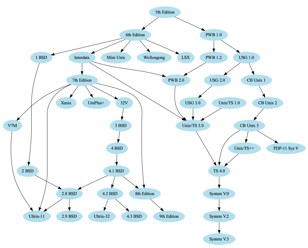

import graphviz


f = graphviz.Digraph('finite_state_machine', filename='fsm.gv')
f.attr(rankdir='LR', size='8,5')


f.attr('node', shape='doublecircle')
f.node('LR_0')
f.node('LR_3')
f.node('LR_4')
f.node('LR_8')


f.attr('node', shape='circle')
f.edge('LR_0', 'LR_2', label='SS(B)')
f.edge('LR_0', 'LR_1', label='SS(S)')
f.edge('LR_1', 'LR_3', label='S($end)')
f.edge('LR_2', 'LR_6', label='SS(b)')
f.edge('LR_2', 'LR_5', label='SS(a)')
f.edge('LR_2', 'LR_4', label='S(A)')
f.edge('LR_5', 'LR_7', label='S(b)')
f.edge('LR_5', 'LR_5', label='S(a)')
f.edge('LR_6', 'LR_6', label='S(b)')
f.edge('LR_6', 'LR_5', label='S(a)')
f.edge('LR_7', 'LR_8', label='S(b)')
f.edge('LR_7', 'LR_5', label='S(a)')
f.edge('LR_8', 'LR_6', label='S(b)')
f.edge('LR_8', 'LR_5', label='S(a)')


f.view()

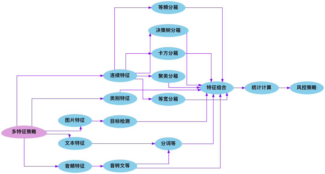
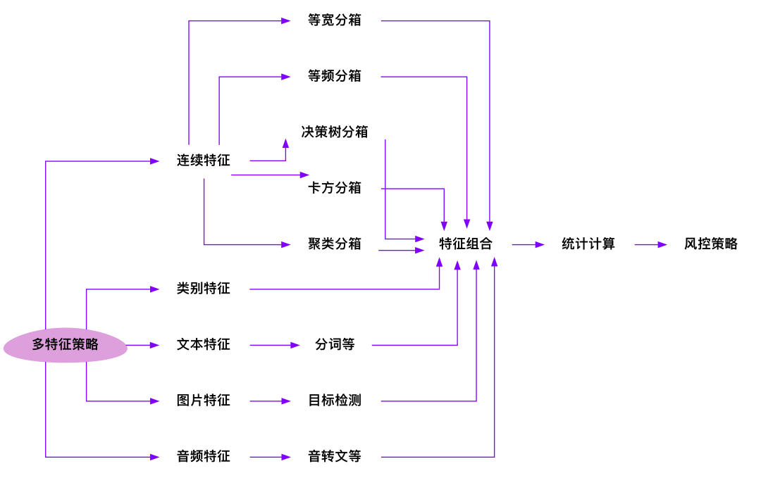
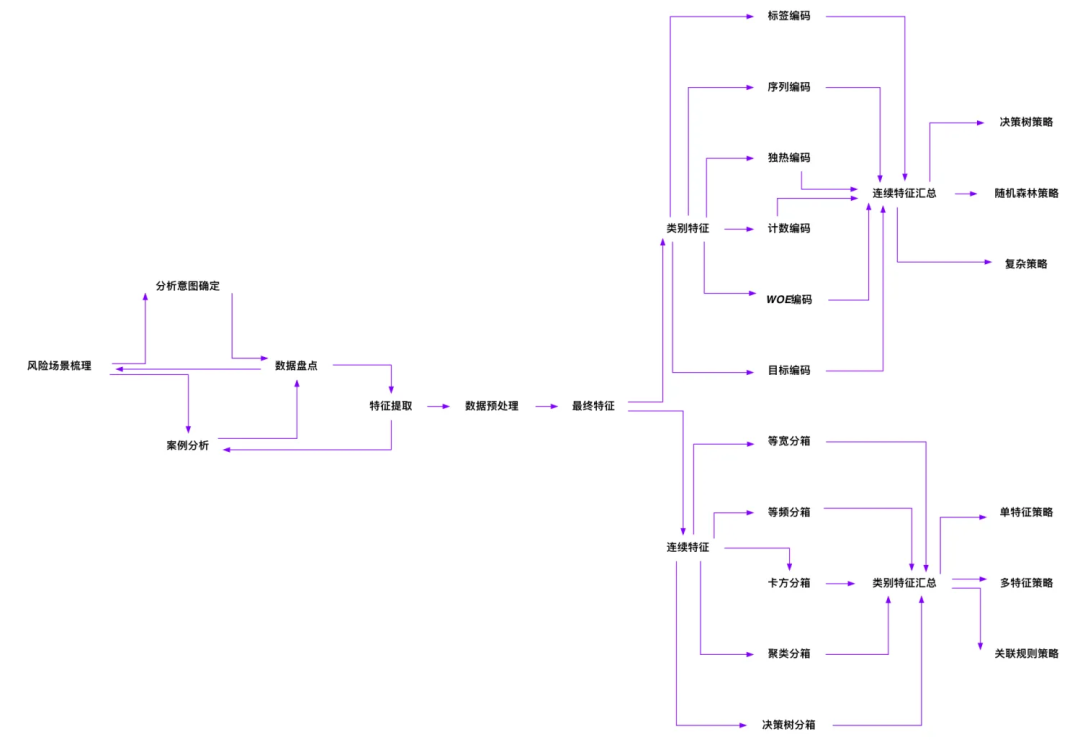
多特征策略挖掘流程

Rule ='多特征策略'


FeaA = '连续特征'
FeaB = '类别特征'
FeaC = '文本特征'
FeaD = '图片特征'
FeaE = '音频特征'




method1 = '等宽分箱'
method2 = '等频分箱'
method3 = '决策树分箱'
method4 = '卡方分箱'
method5 = '聚类分箱'


method6 = '分词等'
method7 = '目标检测'
method8 = '音转文等'


stat = '统计计算'
rest = '风控策略'




Combine = '特征组合'


nodes = [FeaA, FeaB,FeaC,FeaD,FeaE,stat, rest, method1, method2, method3, method4,method5,method6,method7,method8,combine]




import pygraphviz as pgv


# 创建图
G = pgv.AGraph(directed=True, 
               strict=False, 
               ranksep=0.46,#不同级节点最小间距 
               nodesep=0.42,#同级节点最小间距 
               splines="ortho", #可选 ortho (直角), polyline (折线), spline (曲线), line (线条), none (无)
               rankdir='LR',
               concentrate=True
              )




# 添加节点 - 根节点
G.add_node(Rule,
           color="#DDA0DD", 
           style="filled",
           fontname="times bold italic" ,
           shape='egg'
          )


# 添加节点 - 其他节点 #ffffff
G.add_nodes_from(nodes, color="#87CEEB",style="filled",fontname="times bold italic")




# 添加边
G.add_edges_from(
[
[Rule, FeaA],
[Rule, FeaB], 
[Rule, FeaC],
[Rule, FeaD], 
[Rule, FeaE], 
[FeaA, method1], 
[FeaA, method2],
[FeaA, method3], 
[FeaA, method4], 
[FeaA, method5], 




[FeaC, method6], 
[FeaD, method7], 
[FeaE, method8],


[method8, method6],


[FeaB,Combine],  
[method1, Combine],[method2, Combine], [method3, Combine], [method4, Combine],
[method5,Combine],[method6,Combine],[method7,Combine],[method8,Combine],


[Combine,stat],[stat,rest]


],
color="#7F01FF", arrowsize=0.8
)


# 设置图的尺寸 分辨率
G.graph_attr.update(dpi='800')  # 设置分辨率


# 导出图形
G.layout()
G.draw("多特征策略.png", prog="dot")


# 图片图形
from IPython.display import Image
display(Image(filename="多特征策略.png"))

风控策略总体流程

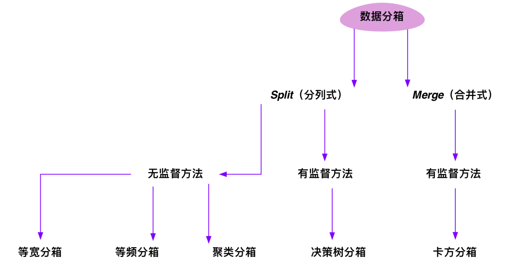
分箱方法

因果关系图

import pygraphviz as pgv


G = pgv.AGraph(directed=True, strict=False, ranksep=0.2, splines="spline", concentrate=True)


# 设置节点标签
nodeA = "Police\nIntelligence"
nodeB = "Police Station"
nodeC = "Criminal Action"
nodeD = "Incidents"
nodeE = "Police Dockets"
nodeF = "Control Room\nAwareness"
nodeG = "Patroller Information"
nodeH = "Patroller Awareness"


# 添加节点
G.add_nodes_from([nodeA, nodeB, nodeC, nodeD, nodeE, nodeF, nodeG, nodeH],
                 color="#ffffff", fontname="times bold italic")


# 添加边
G.add_edges_from([[nodeA, nodeB], [nodeA, nodeF], [nodeB, nodeC], [nodeC, nodeD],
                  [nodeC, nodeG], [nodeD, nodeE], [nodeD, nodeG], [nodeE, nodeA],
                  [nodeF, nodeA], [nodeF, nodeG], [nodeF, nodeH], [nodeG, nodeF],
                  [nodeH, nodeG]], color="#7F01FF", arrowsize=0.8)


# 导出图形
G.layout()
G.draw("因果关系图.png", prog="dot")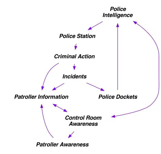

因子相关性图

import pygraphviz as pgv


G = pgv.AGraph(directed=True, rankdir="TB")


# 设置节点标签
Root = "道路交通流畅"
negative_1 = "平均延误时间"
negative_2 = "负荷度"
negative_3 = "小区位置"
negative_4 = "相对延误率"
negative_5 = "房屋密度"
negative_6 = "人口密度"
negative_7 = "总延误率"
negative_8 = "排队率"
negative_9 = "行驶时间"
positive_1 = "通行能力"
positive_2 = "公路层级"
positive_3 = "路网结构"
positive_4 = "行驶速度"
positive_5 = "路网长度"
positive_6 = "小区面积"
positive_7 = "内部道路密度"
positive_8 = "路网密度"


# 添加节点
G.add_node(Root, style="filled", shape="box3d", color="#feb64d")
for negative in [eval(_) for _ in dir() if _.startswith("negative")]:
    G.add_node(negative, style="filled", shape="ellipse", color="#CFDBF6")


for positive in [eval(_) for _ in dir() if _.startswith("positive")]:
    G.add_node(positive, style="filled", shape="ellipse", color="#B4E7B7")


# 添加边
G.add_edges_from([[Root, negative_1], [Root, negative_6], [Root, negative_8], [Root, negative_9],
                  [negative_1, negative_2], [negative_1, negative_7], [negative_2, negative_3],
                  [negative_2, negative_7], [negative_3, negative_4], [negative_8, negative_9],
                  [positive_2, negative_5], [positive_3, negative_4], [positive_4, negative_5]],
                 color="#B4DBFF", style="dashed", penwidth=1.5)


G.add_edges_from([[Root, positive_1], [Root, positive_8], [negative_5, negative_4],
                  [negative_6, positive_4], [negative_5, positive_4], [negative_9, positive_5],
                  [positive_1, positive_2], [positive_2, positive_3], [positive_6, positive_5],
                  [positive_7, positive_6], [positive_8, positive_7]],
                 color="#B4E7B7", style="dashed", penwidth=1.5)


# 导出图形
G.layout()
G.draw("因子相关性图.png", prog="dot")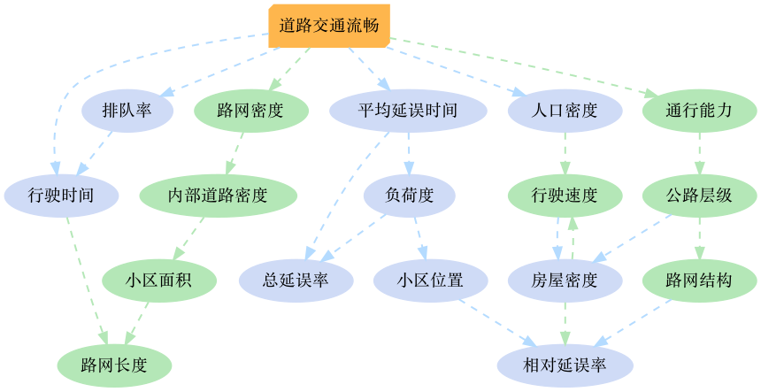

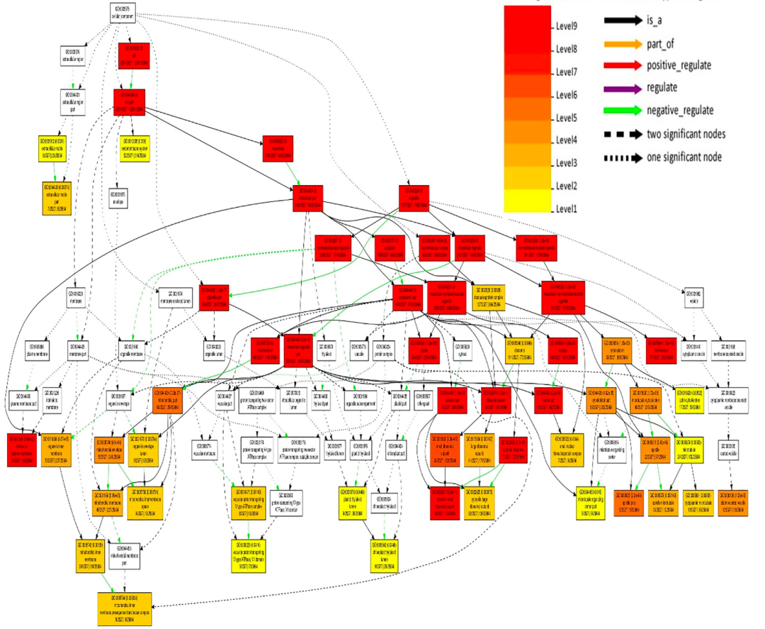
更复杂的案例

往期精彩回顾




适合初学者入门人工智能的路线及资料下载(图文+视频)机器学习入门系列下载机器学习及深度学习笔记等资料打印《统计学习方法》的代码复现专辑

• 交流群

欢迎加入机器学习爱好者微信群一起和同行交流，目前有机器学习交流群、博士群、博士申报交流、CV、NLP等微信群，请扫描下面的微信号加群，备注：”昵称-学校/公司-研究方向“，例如：”张小明-浙大-CV“。请按照格式备注，否则不予通过。添加成功后会根据研究方向邀请进入相关微信群。请勿在群内发送广告，否则会请出群，谢谢理解~（也可以加入机器学习交流qq群772479961）