


文章目录
说明
闵老师的文章链接: 日撸 Java 三百行(总述)_minfanphd的博客-CSDN博客
自己也把手敲的代码放在了github上维护:https://github.com/fulisha-ok/sampledata
1. Day63-65 AdaBoosting算法
1 AdaBoostin举例
AdaBoost算法是一种集成学习算法,是Boosting算法中的一种,通过组合多个弱分类器来构建一个强分类器。因为我也是第一次接触这个算法,直接去看一些算法以及公式,感觉还是有点吃力,所以我结合网上看的例子,自以及己也模拟一个例子先手动过一遍这个算法过程,然后再去学习他的理论知识。(其中的计算结果我是通过文章的代码计算所得的),如果遇到一些概念不懂,我们先假装自己懂,看完例子再去看理论,于我而言,蛮有用的。(若有问题,欢迎指正~)
1.1数据样本
我把原来iris.aff文件的150个缩减为12个数据,数据如下:一共有4种特征,3个类别,12个数据集。
@RELATION iris

@ATTRIBUTE sepallength	REAL
@ATTRIBUTE sepalwidth 	REAL
@ATTRIBUTE petallength 	REAL
@ATTRIBUTE petalwidth	REAL
@ATTRIBUTE class 	{Iris-setosa,Iris-versicolor,Iris-virginica}

@DATA
5.1,3.5,1.4,0.2,Iris-setosa
4.9,3.0,1.4,0.2,Iris-setosa
4.7,3.2,1.3,0.2,Iris-setosa
4.6,3.1,1.5,0.2,Iris-setosa
5.0,3.6,1.4,0.2,Iris-setosa
5.4,3.9,1.7,0.4,Iris-setosa
7.0,3.2,4.7,1.4,Iris-versicolor
6.4,3.2,4.5,1.5,Iris-versicolor
6.9,3.1,4.9,1.5,Iris-versicolor
5.5,2.3,4.0,1.3,Iris-versicolor
6.5,2.8,4.6,1.5,Iris-versicolor
5.7,2.8,4.5,1.3,Iris-versicolor
6.3,3.3,6.0,2.5,Iris-virginica
5.8,2.7,5.1,1.9,Iris-virginica
7.1,3.0,5.9,2.1,Iris-virginica
6.3,2.9,5.6,1.8,Iris-virginica
6.5,3.0,5.8,2.2,Iris-virginica
7.6,3.0,6.6,2.1,Iris-virginica
1.2 举例过程
先初始化这12个数据集的权重: 1 N \frac{1}{N} N1
| 索引 | 0 | 1 | 2 | 3 | 4 | 5 | 6 | 7 | 8 | 9 | 10 | 11 |
|---|---|---|---|---|---|---|---|---|---|---|---|---|
| 权重 | 0.083 | 0.083 | 0.083 | 0.083 | 0.083 | 0.083 | 0.083 | 0.083 | 0.083 | 0.083 | 0.083 | 0.083 |
由于我们有三个类别,对于属性的选择我们都是随机选择属性来进行训练。我们的基学习器采用的是树桩分类器。(树桩分类器是决策树的一种特殊形式,它只包含一个根结点和两个叶子结点,相当于把数据按一个阈值一分为二,基类学习器还有我们之前学的KNN,贝叶斯算法等。)
前提:我们在每次学习的时候,基类学习器G(x)的值我们用+1来表示与我们预期相符合(正类别);-1来表示与我们预期不符合(负类别)
- 第一个弱学习器(基类学习器)
随机选择的属性为sepallength
| 索引 | 0 | 1 | 2 | 3 | 4 | 5 | 6 | 7 | 8 | 9 | 10 | 11 |
|---|---|---|---|---|---|---|---|---|---|---|---|---|
| 属性 | 5.1 | 4.9 | 4.7 | 4.6 | 7.0 | 6.4 | 6.9 | 5.5 | 6.3 | 5.8 | 7.1 | 6.3 |
| 权重w1 | 0.083 | 0.083 | 0.083 | 0.083 | 0.083 | 0.083 | 0.083 | 0.083 | 0.083 | 0.083 | 0.083 | 0.083 |
| 正确结果 y 1 ( x ) y_{1}(x) y1(x) | 0 | 0 | 0 | 0 | 1 | 1 | 1 | 1 | 2 | 2 | 2 | 2 |
| 预测结果 G 1 ( x ) G_{1}(x) G1(x) | 0 | 0 | 0 | 0 | 1 | 1 | 1 | 1 | 1 | 1 | 1 | 1 |
我们的最佳分割点bestCut=5.3; leftLeafLabel = 0 ; rightLeafLabel = 1;
误差率
e
1
=
0.083
+
0.083
+
0.083
+
0.083
=
0.3333
e1=0.083 + 0.083 + 0.083 + 0.083 = 0.3333
e1=0.083+0.083+0.083+0.083=0.3333
误差系数:
α
1
=
1
2
log
1
−
e
1
e
1
=
0.3465
\alpha _{1}=\frac{1}{2}\log \frac{1-e_{1}}{e_{1}}=0.3465
α1=21loge11−e1=0.3465
训练数据的准确率:0.6667
弱学习器
G
1
(
x
)
G_{1}(x)
G1(x):
G
1
(
x
)
=
{
0
,
x < 5.3
1
,
x > 5.3
G_{1}(x)= \begin{cases} 0, & \text {x < 5.3} \\ 1, & \text{x > 5.3} \end{cases}
G1(x)={0,1,x < 5.3x > 5.3
- 第二个弱学习器(基类学习器)
随机选择的属性为petallength
| 索引 | 0 | 1 | 2 | 3 | 4 | 5 | 6 | 7 | 8 | 9 | 10 | 11 |
|---|---|---|---|---|---|---|---|---|---|---|---|---|
| 属性 | 1.4 | 1.4 | 1.3 | 1.5 | 4.7 | 4.5 | 4.9 | 4.0 | 6.0 | 5.1 | 5.9 | 5.6 |
| 权重w2 | 0.062 | 0.062 | 0.062 | 0.062 | 0.062 | 0.062 | 0.062 | 0.062 | 0.125 | 0.125 | 0.125 | 0.125 |
| 正确结果 y 2 ( x ) y_{2}(x) y2(x) | 0 | 0 | 0 | 0 | 1 | 1 | 1 | 1 | 2 | 2 | 2 | 2 |
| 预测结果 G 2 ( x ) G_{2}(x) G2(x) | 0 | 0 | 0 | 0 | 2 | 2 | 2 | 2 | 2 | 2 | 2 | 2 |
我们的阈值取值为: 2.75; leftLeafLabel = 0 ; rightLeafLabel = 2;
误差权重之和
e
2
=
0.062
+
0.062
+
0.062
+
0.062
=
0.249
e2=0.062 + 0.062 + 0.062 + 0.062 = 0.249
e2=0.062+0.062+0.062+0.062=0.249
误差系数:
α
2
=
1
2
log
1
−
e
2
e
2
=
0.5493
\alpha _{2}=\frac{1}{2}\log \frac{1-e_{2}}{e_{2}}=0.5493
α2=21loge21−e2=0.5493
训练数据的准确率:0.6666
弱学习器
G
2
(
x
)
G_{2}(x)
G2(x):
G
2
(
x
)
=
{
0
,
x < 2.75
2
,
x >2.75
G_{2}(x)= \begin{cases} 0, & \text {x < 2.75} \\ 2, & \text{x >2.75} \end{cases}
G2(x)={0,2,x < 2.75x >2.75
- 第三个弱学习器(基类学习器)
随机选择的属性为petalwidth
| 索引 | 0 | 1 | 2 | 3 | 4 | 5 | 6 | 7 | 8 | 9 | 10 | 11 |
|---|---|---|---|---|---|---|---|---|---|---|---|---|
| 属性 | 0.2 | 0.2 | 0.2 | 0.2 | 1.4 | 1.5 | 1.5 | 1.3 | 2.5 | 1.9 | 2.1 | 1.8 |
| 权重w3 | 0.041 | 0.041 | 0.041 | 0.041 | 0.125 | 0.125 | 0.125 | 0.125 | 0.083 | 0.083 | 0.083 | 0.083 |
| 正确结果 y 3 ( x ) y_{3}(x) y3(x) | 0 | 0 | 0 | 0 | 1 | 1 | 1 | 1 | 2 | 2 | 2 | 2 |
| 预测结果 G 3 ( x ) G_{3}(x) G3(x) | 1 | 1 | 1 | 1 | 1 | 1 | 1 | 1 | 2 | 2 | 2 | 2 |
我们的阈值取值为:1.65; leftLeafLabel = 1 ; rightLeafLabel = 2;
误差权重之和
e
3
=
0.041
+
0.041
+
0.041
+
0.041
=
0.166
e3=0.041 + 0.041 + 0.041 + 0.041 = 0.166
e3=0.041+0.041+0.041+0.041=0.166
误差系数:
α
3
=
1
2
log
1
−
e
3
e
3
=
0.8047
\alpha _{3}=\frac{1}{2}\log \frac{1-e_{3}}{e_{3}}=0.8047
α3=21loge31−e3=0.8047
训练数据的准确率:1.0
弱学习器
G
3
(
x
)
G_{3}(x)
G3(x):
G
3
(
x
)
=
{
1
,
x < 1.65
2
,
x > 1.65
G_{3}(x)= \begin{cases} 1, & \text {x < 1.65} \\ 2, & \text{x > 1.65} \end{cases}
G3(x)={1,2,x < 1.65x > 1.65
我针对第三次的学习来计算他们的准确率:
假设给出的实例:5.1,3.5,1.4,0.2,Iris-setosa
他在第一次基类学习器中预测类别为0: 则第一个类别累加误差系数 0.3465
他在第二次基类学习器中预测类别为0: 则第一个类别累加0.5493后为0.8958
他在第一次基类学习器中预测类别为1: 则第二个类别为:0.8047
故第一个实例的预测类别概率为:[0.8958797346140277, 0.8047189562170501, 0.0]可知预测的为类别0
其他11个实例依次预测的类别为:
[0.8958797346140277, 0.8047189562170501, 0.0]
[0.8958797346140277, 0.8047189562170501, 0.0]
[0.8958797346140277, 0.8047189562170501, 0.0]
[0.0, 1.1512925464970227, 0.549306144334055]
[0.0, 1.1512925464970227, 0.549306144334055]
[0.0, 1.1512925464970227, 0.549306144334055]
[0.0, 1.1512925464970227, 0.549306144334055]
[0.0, 0.34657359027997264, 1.3540251005511053]
[0.0, 0.34657359027997264, 1.3540251005511053]
[0.0, 0.34657359027997264, 1.3540251005511053]
[0.0, 0.34657359027997264, 1.3540251005511053]
结合上面的例子,就可以来学习理论知识了:
2. 理论知识
算法步骤(我参考了网上的帖子,这里梳理出来是为了方便以后回顾)
- 1. 假设训练集样本是这样的:
T = ( x 1 , y 1 ) , ( x 2 , y 2 ) . . . . . ( x m , y m ) T={({x_{1}, y_{1}}), ({x_{2}, y_{2}})..... ({x_{m}, y_{m}})} T=(x1,y1),(x2,y2).....(xm,ym)
y i {y_{i}} yi 的取值如果在一个二分类问题中,可以取值+1和-1,在多类别问题中,要根据情况而定。如我们在上面的例子中,表示样本 x i x_{i} xi所属的类别
- 2. 第m个弱学习器的各个数据的权重是:
D k = ( w m 1 , w m 2 , w m 3 . . . . w m i ) D_{k}=(w_{m1},w_{m2},w_{m3}....w_{mi}) Dk=(wm1,wm2,wm3....wmi)
其中初始化的权重为如下:N为样本数量
D 1 = ( w 11 , w 12 , w 13 . . . . ) , w 1 i = 1 N , i = 1 , 2 , 3 , 4... N D_{1}=(w_{11},w_{12},w_{13}....), w_{1i}=\frac{1}{N}, i=1,2,3,4...N D1=(w11,w12,w13....),w1i=N1,i=1,2,3,4...N - 3. 第m个学习器 G m ( x ) G_{m}(x) Gm(x)
G m ( x ) G_{m}(x) Gm(x)其取值只能有两个(正类别+1和负类别-1),而在多类别问题中,也依情况而定,我在上面例子中去的是具体的类别。
-
4. G m ( x ) G_{m}(x) Gm(x)在训练数据集上的误差率(即失败样本数*样本权重之和):
e m = P ( G m ( x i ) ≠ y i ) = ∑ i = 1 m w m i I ( G m ( x i ) ≠ y i ) e_{m}=P(G_{m}(x_{i})\neq y_{i})=\sum_{i=1}^{m}w_{mi}I(G_{m}(x_{i})\neq y_{i}) em=P(Gm(xi)=yi)=i=1∑mwmiI(Gm(xi)=yi)
其中 I ( G m ( x i ) ≠ y i ) { I(G_m(x_i) ≠ y_i) } I(Gm(xi)=yi)的值为1,即预测的结果与实际结果不符合 -
5.计算 G m ( x ) G_{m}(x) Gm(x)的权重系数:
(由公式可以看出,当误差率越小的弱分类器,在最后的强分类器中贡献越大)
α m = 1 2 log 1 − e m e m \alpha _{m}=\frac{1}{2}\log \frac{1-e_{m}}{e_{m}} αm=21logem1−em
权重系数在最终分类器中会发挥作用,当值越大对最终的影响就较大;同时权重系数还会影响下一次权重更新。 -
6.更新权重的公式:
已知: D m = ( w m 1 , w m 2 , w m 3 . . . . w m i ) D_{m}=(w_{m1},w_{m2},w_{m3}....w_{mi}) Dm=(wm1,wm2,wm3....wmi)的权重,现在计算第m+1个样本集的权重
w
m
+
1
,
i
=
w
m
i
Z
m
e
x
p
(
−
α
m
y
i
G
m
(
x
i
)
)
w_{m+1,i}=\frac{w_{mi}}{Z_{m}}exp(-\alpha _{m}y_{i}G_{m}(x_{i}))
wm+1,i=Zmwmiexp(−αmyiGm(xi))
其中我们可以简化公式:
w
m
+
1
,
i
=
{
w
m
i
Z
m
1
e
α
m
,
G
m
(
x
i
)
=
y
i
→
(
G
m
(
x
i
)
∗
y
i
=
1
)
w
m
i
Z
m
e
α
m
,
G
m
(
x
i
)
≠
y
i
→
(
G
m
(
x
i
)
∗
y
i
=
−
1
)
w_{m+1,i} = \begin{cases} \frac{w_{mi}}{Z_{m}}\frac{1}{e^{\alpha_{m}}}, & G_{m}(x_{i})=y_{i} \rightarrow (G_{m}(x_{i})*y_{i}=1)\\ \frac{w_{mi}}{Z_{m}}e^{\alpha_{m}}, & G_{m}(x_{i})\neq y_{i} \rightarrow (G_{m}(x_{i})*y_{i}=-1)\\ \end{cases}
wm+1,i={Zmwmieαm1,Zmwmieαm,Gm(xi)=yi→(Gm(xi)∗yi=1)Gm(xi)=yi→(Gm(xi)∗yi=−1)
(
G
m
(
x
i
)
∗
y
i
=
1
)
(G_{m}(x_{i})*y_{i}=1)
(Gm(xi)∗yi=1)的前提是
G
m
(
x
i
)
和
y
i
G_{m}(x_{i})和y_{i}
Gm(xi)和yi取值在+1和-1,而实际上我觉得这个公式要描述的意思就可以理解为:如果预测结果一致就为1,预测结果不一致为-1。就如例子上面我们有3个类别,并没有按+1,-1去计算,所以要依情况而定,但核心思想不变!其中
Z
k
Z_{k}
Zk是规范化因子
Z
k
=
∑
i
=
1
m
w
k
i
e
x
p
(
−
α
k
y
i
G
k
(
x
i
)
)
Z_{k}=\sum_{i=1}^{m}w_{ki}exp(-\alpha_{k}y_{i}G_{k}(x_{i}))
Zk=i=1∑mwkiexp(−αkyiGk(xi))
从上面的是公式,我们可以知道在计算
w
m
+
1
,
i
w_{m+1,i}
wm+1,i 的值时,
α
m
\alpha _{m}
αm的值肯定是大于0的 则
e
α
m
e^{\alpha _{m}}
eαm的值一定是大于1,当我们在第m+1次更新权重时,如果在第m次样本被正确分类(
(
G
m
(
x
i
)
=
y
i
(G_{m}(x_{i})=y_{i}
(Gm(xi)=yi),则他在第m+1次时权重就会变小,而若被错误分类(
G
m
(
x
i
)
≠
y
i
G_{m}(x_{i})\neq y_{i}
Gm(xi)=yi),则在第m+1次时权重就会变大 (因为在上一次已经被错误分类了,那么我在这一次的分类中我需要更重视错误分类的,所以就把权重要调大!)
3. 总结
结合上面的例子和公式,去看这个图就非常的生动,我们训练多个弱分类器(串行的),每一次弱分类器中数据的权重都是根据上一次的权重,误差概率和误差系数来更新,经过多次训练后我们最终形成一个最终的强分类器,我们预测类别是就通过计算多个弱分类器的一个加权和来预测那个类别概率最大(并行的)
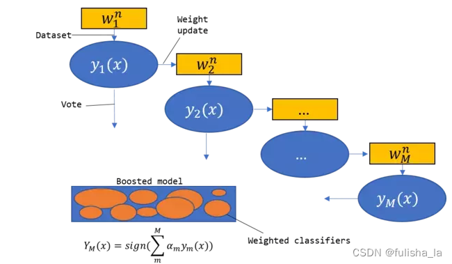
AdaBoosting算法在每一次的弱分类器的训练中,实际上是一个二分类的问题。但是我们在上面的例子中,他实际上是一个多类别问题,那我们也可以通过这个算法来实现。我们的实现是对每个基本分类器都选择两个类别。在预测阶段,通过对这些基本分类器的预测结果进行投票,选择概率最大的。
2. 代码理解
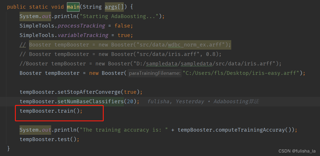
我从Booster类去理解代码。下面是Booster的main方法,而最核心的东西就是train()方法,其中我们设置了训练的次数是20个。
下面是train的核心代码
public void train() {
// Step 1. Initialize.
WeightedInstances tempWeightedInstances = null;
double tempError;
numClassifiers = 0;
SimpleTools.processTrackingOutput("Booster.train() Step 1\r\n");
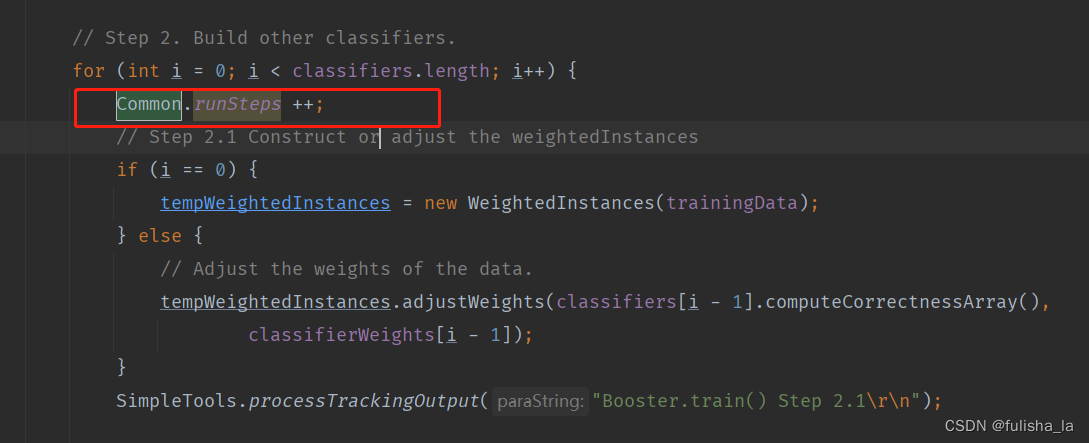
// Step 2. Build other classifiers.
for (int i = 0; i < classifiers.length; i++) {
Common.runSteps ++;
// Step 2.1 Construct or adjust the weightedInstances
if (i == 0) {
tempWeightedInstances = new WeightedInstances(trainingData);
} else {
// Adjust the weights of the data.
tempWeightedInstances.adjustWeights(classifiers[i - 1].computeCorrectnessArray(),
classifierWeights[i - 1]);
}
SimpleTools.processTrackingOutput("Booster.train() Step 2.1\r\n");
// Step 2.2 Train the next classifier.
switch (baseClassifierType) {
case STUMP_CLASSIFIER:
classifiers[i] = new StumpClassifier(tempWeightedInstances);
break;
case BAYES_CLASSIFIER:
classifiers[i] = new BayesClassifier(tempWeightedInstances);
break;
case Gaussian_CLASSIFIER:
classifiers[i] = new GaussianClassifier(tempWeightedInstances);
break;
default:
System.out.println(
"Internal error. Unsupported base classifier type: " + baseClassifierType);
System.exit(0);
}
classifiers[i].train();
SimpleTools.processTrackingOutput("Booster.train() Step 2.2\r\n");
// tempAccuracy = classifiers[i].computeTrainingAccuracy();
//计算加权错误率
tempError = classifiers[i].computeWeightedError();
// Set the classifier weight. 弱分类器的权重
classifierWeights[i] = 0.5 * Math.log(1 / tempError - 1);
if (classifierWeights[i] < 1e-6) {
classifierWeights[i] = 0;
}
// SimpleTools.variableTrackingOutput("Booster.train()");
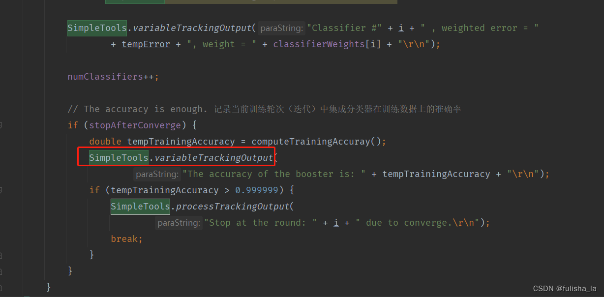
SimpleTools.variableTrackingOutput("Classifier #" + i + " , weighted error = "
+ tempError + ", weight = " + classifierWeights[i] + "\r\n");
numClassifiers++;
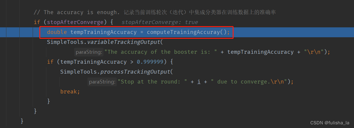
// The accuracy is enough. 记录当前训练轮次(迭代)中集成分类器在训练数据上的准确率
if (stopAfterConverge) {
double tempTrainingAccuracy = computeTrainingAccuray();
SimpleTools.variableTrackingOutput(
"The accuracy of the booster is: " + tempTrainingAccuracy + "\r\n");
if (tempTrainingAccuracy > 0.999999) {
SimpleTools.processTrackingOutput(
"Stop at the round: " + i + " due to converge.\r\n");
break;
}
}
}
}
其中的for循环则是训练的次数,我就以一次训练过程来学习整个内容。通过Booster类中的train方法为入口,去了解这个方法中调用其他类的一些方法。
1. WeightedInstances类
在WeightedInstances类中最重要的方法就是adjustWeights,调整数据样本的权重。
下面这个是Booster方法中train()中调用WeightedInstances类的方法:

- new WeightedInstances(trainingData)
这里的方法是更新数据集样本中每个数据的权重,其中new WeightedInstances(trainingData)方法是在第一次训练时,初始化权重的值。初始化权重为 1 N \frac{1}{N} N1,N为样本的个数
	public WeightedInstances(Instances paraInstances) {
		super(paraInstances);
		setClassIndex(numAttributes() - 1);

		// Initialize weights
		weights = new double[numInstances()];
		double tempAverage = 1.0 / numInstances();
		for (int i = 0; i < weights.length; i++) {
			Common.runSteps ++;
			weights[i] = tempAverage;
		}
		SimpleTools.variableTrackingOutput("Instances weights are: " + Arrays.toString(weights));
	}
- adjustWeights方法
- 入参paraCorrectArray是上一次训练的预测结果(bool值:true or false)
- 入参paraAlpha 上一次训练的误差系数
α
m
\alpha _{m}
αm
循环数据样本,更新每个数据的权重值(weights[i]的值):
若在上一次训练中预测结果为true,则weights[i] = weights[i] * e α m e^{\alpha _{m}} eαm;
若预测结果为false,则weights[i] = weights[i] * 1 e α m \frac{1}{e^{\alpha _{m}}} eαm1
最后的循环中进行归一化操作。
public void adjustWeights(boolean[] paraCorrectArray, double paraAlpha) {
		// Step 2. Calculate alpha.
		double tempIncrease = Math.exp(paraAlpha);

		// Step 3. Adjust.
		double tempWeightsSum = 0; // For normalization.
		for (int i = 0; i < weights.length; i++) {
			Common.runSteps ++;
			if (paraCorrectArray[i]) {
				weights[i] /= tempIncrease;
			} else {
				weights[i] *= tempIncrease;
			} // Of if
			tempWeightsSum += weights[i];
		}

		// Step 4. Normalize.
		for (int i = 0; i < weights.length; i++) {
			Common.runSteps ++;
			weights[i] /= tempWeightsSum;
		}

		SimpleTools.variableTrackingOutput(
				"After adjusting, instances weights are: " + Arrays.toString(weights));
	}
2. 选择基分类器并进行训练(树桩分类器)
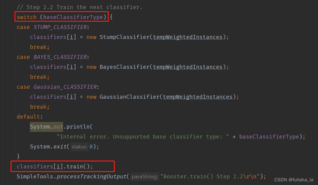
这里选择基分类器为树桩分类器(StumpClassifier类),如下是StumpClassifier类的train()方法。
具体的实现步骤是:
- 因为特征值较多,这里采用随机的方法,随机选择。(java的Random方法)
- tempValuesArray记录所选择特征值的取值并进行排序。(Arrays.sort方法)
- 迭代所有的数据,找出最佳的分割点bestCut,以及左右子结点的类别取值(leftLeafLabel,rightLeafLabel)
每一次训练,遍历所有的特征值,寻找可能取得的分割点进行计算,以获取最佳的分割点(选取分割点的方法有很多,在文章中的分割点是选取的前后两个特征值的平均值,但分割点的选取方式有很多,可以依情况而定) 选择最佳分割点是使划分的两个子集数据误差最小。
@Override
	public void train() {
		// Step 1. Randomly choose an attribute.
		selectedAttribute = Common.random.nextInt(numConditions);

		// Step 2. Find all attribute values and sort.
		double[] tempValuesArray = new double[numInstances];
		for (int i = 0; i < tempValuesArray.length; i++) {
			tempValuesArray[i] = weightedInstances.instance(i).value(selectedAttribute);
		}
		Arrays.sort(tempValuesArray);
		Common.runSteps += (long)(numInstances * Math.log(numInstances) / Math.log(2));

		// Step 3. Initialize, classify all instances as the same with the
		// original cut.
		int tempNumLabels = numClasses;
		double[] tempLabelCountArray = new double[tempNumLabels];
		int tempCurrentLabel;

		// Step 3.1 Scan all labels to obtain their counts.
		for (int i = 0; i < numInstances; i++) {
			Common.runSteps ++;
			// The label of the ith instance
			tempCurrentLabel = (int) weightedInstances.instance(i).classValue();
			tempLabelCountArray[tempCurrentLabel] += weightedInstances.getWeight(i);
		}

		// Step 3.2 Find the label with the maximal count.
		double tempMaxCorrect = 0;
		int tempBestLabel = -1;
		for (int i = 0; i < tempLabelCountArray.length; i++) {
			if (tempMaxCorrect < tempLabelCountArray[i]) {
				tempMaxCorrect = tempLabelCountArray[i];
				tempBestLabel = i;
			}
		}

		// Step 3.3 The cut is a little bit smaller than the minimal value.
		bestCut = tempValuesArray[0] - 0.1;
		leftLeafLabel = tempBestLabel;
		rightLeafLabel = tempBestLabel;

		// Step 4. Check candidate cuts one by one.
		// Step 4.1 To handle multi-class data, left and right.
		double tempCut;
		double[][] tempLabelCountMatrix = new double[2][tempNumLabels];

		for (int i = 0; i < tempValuesArray.length - 1; i++) {
			// Step 4.1 Some attribute values are identical, ignore them.
			if (tempValuesArray[i] == tempValuesArray[i + 1]) {
				continue;
			}
			tempCut = (tempValuesArray[i] + tempValuesArray[i + 1]) / 2;

			// Step 4.2 Scan all labels to obtain their counts wrt. the cut.
			// Initialize again since it is used many times.
			for (int j = 0; j < 2; j++) {
				for (int k = 0; k < tempNumLabels; k++) {
					Common.runSteps ++;
					tempLabelCountMatrix[j][k] = 0;
				}
			}

			for (int j = 0; j < numInstances; j++) {
				Common.runSteps ++;
				// The label of the jth instance
				tempCurrentLabel = (int) weightedInstances.instance(j).classValue();
				if (weightedInstances.instance(j).value(selectedAttribute) < tempCut) {
					tempLabelCountMatrix[0][tempCurrentLabel] += weightedInstances.getWeight(j);
				} else {
					tempLabelCountMatrix[1][tempCurrentLabel] += weightedInstances.getWeight(j);
				}
			}

			// Step 4.3 Left leaf. 记录左叶子结点的数据
			double tempLeftMaxCorrect = 0;
			int tempLeftBestLabel = 0;
			for (int j = 0; j < tempLabelCountMatrix[0].length; j++) {
				Common.runSteps ++;
				if (tempLeftMaxCorrect < tempLabelCountMatrix[0][j]) {
					tempLeftMaxCorrect = tempLabelCountMatrix[0][j];
					tempLeftBestLabel = j;
				}
			}

			// Step 4.4 Right leaf.
			double tempRightMaxCorrect = 0;
			int tempRightBestLabel = 0;
			for (int j = 0; j < tempLabelCountMatrix[1].length; j++) {
				Common.runSteps ++;
				if (tempRightMaxCorrect < tempLabelCountMatrix[1][j]) {
					tempRightMaxCorrect = tempLabelCountMatrix[1][j];
					tempRightBestLabel = j;
				}
			}

			// Step 4.5 Compare with the current best.
			if (tempMaxCorrect < tempLeftMaxCorrect + tempRightMaxCorrect) {
				Common.runSteps ++;
				tempMaxCorrect = tempLeftMaxCorrect + tempRightMaxCorrect;
				bestCut = tempCut;
				leftLeafLabel = tempLeftBestLabel;
				rightLeafLabel = tempRightBestLabel;
			}
		}

		SimpleTools.variableTrackingOutput("Attribute = " + selectedAttribute + ", cut = " + bestCut
				+ ", leftLeafLabel = " + leftLeafLabel + ", rightLeafLabel = " + rightLeafLabel);
	}
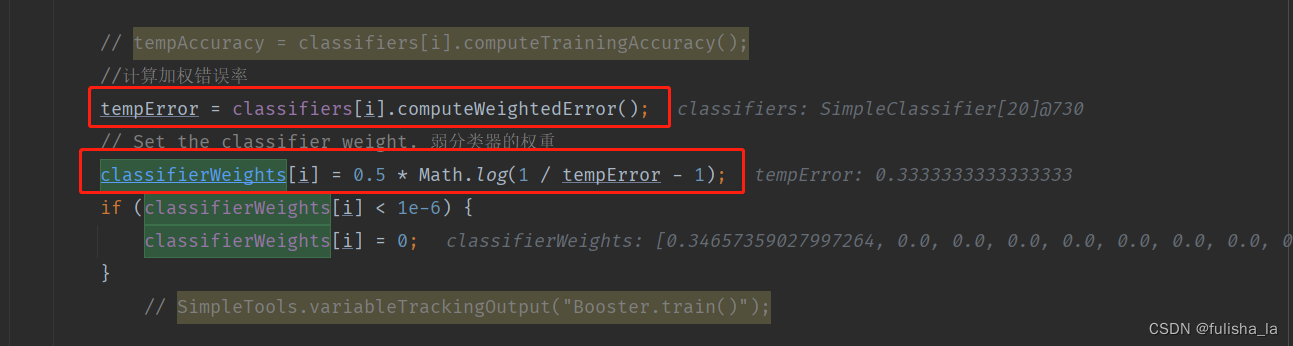
3. 计算误差率和误差系数(树桩分类器)
调用StumpClassifier类的computeWeightedError方法。(实际上这个computeWeightedError方法是公用的,使用的是StumpClassifier的父类SimpleClassifier提供的实现方法)
- 在这个方法中,调用computeCorrectnessArray()获取训练样本在这一次训练中的预测结果和实际结果是否一样,例如下:
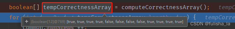
- 计算误差率:失败样本数*样本权重之和
resultError += weightedInstances.getWeight(i); - 计算误差系数(弱分类器的权重)
α
m
=
1
2
log
1
−
e
m
e
m
\alpha _{m}=\frac{1}{2}\log \frac{1-e_{m}}{e_{m}}
αm=21logem1−em
classifierWeights[i] = 0.5 * Math.log(1 / tempError - 1);
public double computeWeightedError() {
		double resultError = 0;
		boolean[] tempCorrectnessArray = computeCorrectnessArray();
		for (int i = 0; i < tempCorrectnessArray.length; i++) {
			Common.runSteps ++;
			if (!tempCorrectnessArray[i]) {
				resultError += weightedInstances.getWeight(i);
			}
		}

		if (resultError < 1e-6) {
			resultError = 1e-6;
		}

		return resultError;
	}
4. 计算精确度
随着训练的次数越来越多,精确度会越来越好,若精确度足够大,就可以跳出训练。
- classify方法
入参为传入的数据实例。 如 5.1,3.5,1.4,0.2,Iris-setosa
第一个for循环累加已经训练的基分类器中的权重系数,第二个for循环选择所有类别中概率最大的即为预测的类别
计算所有训练样本的预测结果与实际结果对比,计算准确率。
从这里也可以看出,当你训练次数越多(即numClassifiers越大),那预测正确的概率也会越大。
public double computeTrainingAccuray() {
		double tempCorrect = 0;

		for (int i = 0; i < trainingData.numInstances(); i++) {
			Common.runSteps ++;
			if (classify(trainingData.instance(i)) == (int) trainingData.instance(i).classValue()) {
				tempCorrect++;
			}
		}

		double tempAccuracy = tempCorrect / trainingData.numInstances();

		return tempAccuracy;
	}

	public int classify(Instance paraInstance) {
		double[] tempLabelsCountArray = new double[trainingData.classAttribute().numValues()];
		for (int i = 0; i < numClassifiers; i++) {
			Common.runSteps ++;
			int tempLabel = classifiers[i].classify(paraInstance);
			tempLabelsCountArray[tempLabel] += classifierWeights[i];
		}

		SimpleTools.variableTrackingOutput(Arrays.toString(tempLabelsCountArray));

		int resultLabel = -1;
		double tempMax = -1;
		for (int i = 0; i < tempLabelsCountArray.length; i++) {
			Common.runSteps ++;
			if (tempMax < tempLabelsCountArray[i]) {
				tempMax = tempLabelsCountArray[i];
				resultLabel = i;
			}
		}

		return resultLabel;
	}
5. 总结
因为这个AdaBosting算法的实现,涉及到不同类中方法的调用,所以需要知道这个算法的一个大致思想以及他的一些理论公式,再去看代码会更容易接受。同时,基分类器这里选择了树桩分类器,还有其他分类器可选。每个分类器的大致思想都是:
- 初始化新训练样本的权重或根据上一次训练结果更新权重
- 选择分类器,并根据分类器进行训练并计算在这一次训练中的错误率以及分类器的权重系数
3. java知识
在这个代码的实现中,用了一些java的基础知识
1. 抽象类
SimpleClassifier类。方法包含的成员变量和方法
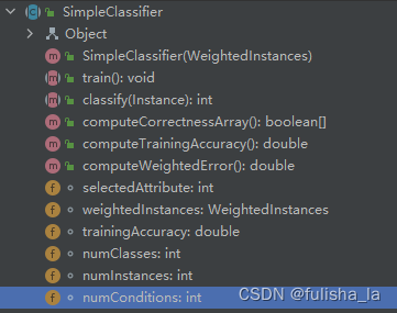
抽象类不能被实例只能被继承。抽象类定义的是一组通用相关的属性和方法,并可以提供一些默认的实现,但SimpleClassifier这个类是无法实例化的(即不能被new)他主要的特点有:
- 1.无法被实例化
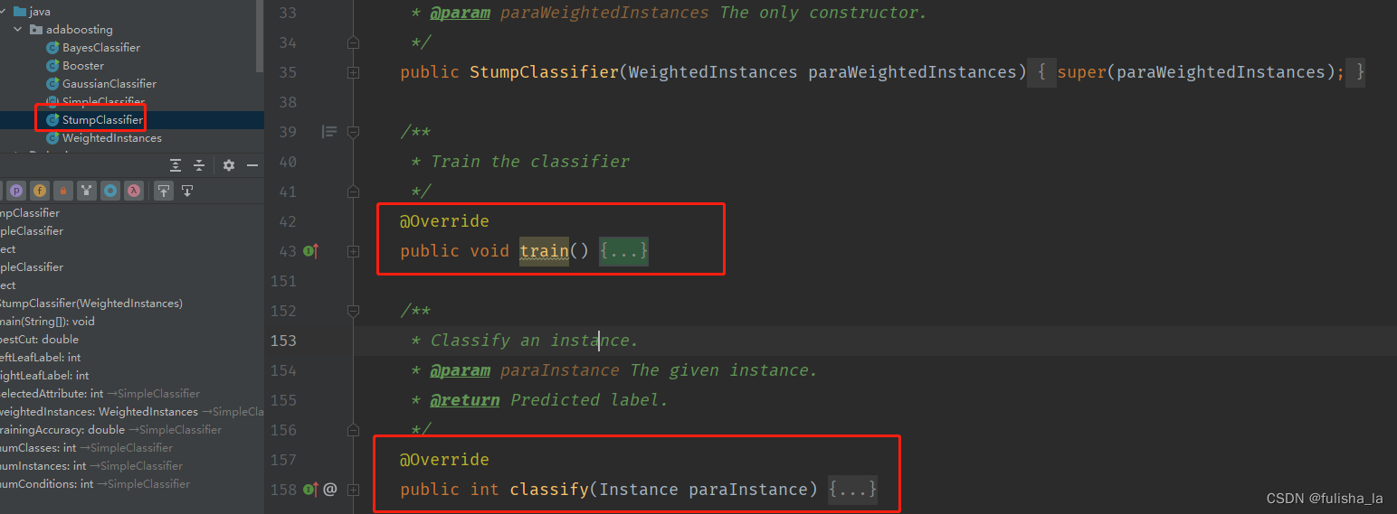
- 2.可以包含抽象方法:抽象方法是没有实现的,且要用abstract关键字声明,子类继承SimpleClassifier必须要实现这两个方法。如SimpleClassifier类的这两个方法。StumpClassifier类集成了SimpleClassifier类,且实现了这两个方法、
	/**
	 * Train the classifier.
	 */
	public abstract void train();

	/**
	 * Classify an instance.
	 * @param paraInstance The given instance.
	 * @return Predicted label.
	 */
	public abstract int classify(Instance paraInstance);
- 可以包含非抽象方法:这些方法包含具体的实现,子类可以继承这些方法,当然也可以重写。例如SimpleClassifier类中的computeCorrectnessArray(),computeTrainingAccuracy(),computeWeightedError()方法
- 可以包含成员变量和构造方法。
2. static关键字
在今天的代码中,有Common类和SimpleTools类两个公共类,其中的成员变量和方法都是用static关键字修饰的,将在类的所有实例之间共享,即使没有创建类的实例对象,也可以直接通过类名来访问该成员变量。静态变量在内存中只有一份拷贝,被所有实例共享。通常用于表示类的共享数据或常量。
如代码中:
3. 静态代码块
在今天的代码中,Common类中有静态代码块,如下:
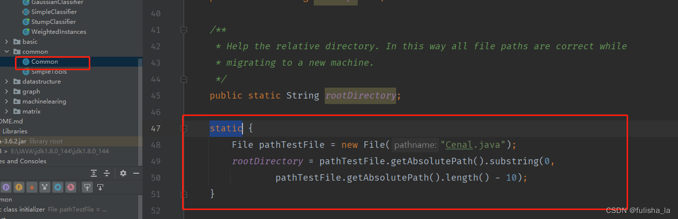
静态代码块在类加载的过程中执行,且只执行一次。他的作用主要是在类加载时执行一些初始化操作。(所以一些初始化的操作或变量可以放在这个里面执行)


 3万+
3万+


 被折叠的 条评论
为什么被折叠?
被折叠的 条评论
为什么被折叠?
 到【灌水乐园】发言


