机器学习论文：《LightGBM: A Highly Efficient Gradient Boosting Decision Tree》

翻译自《LightGBM: A Highly Efficient Gradient Boosting Decision Tree》

摘要

Gradient Boosting Decision Tree (GBDT) is a popular machine learning algorithm, and has quite a few effective implementations such as XGBoost and pGBRT. Although many engineering optimizations have been adopted in these implementations, the efficiency and scalability are still unsatisfactory when the feature dimension is high and data size is large. A major reason is that for each feature, they need to scan all the data instances to estimate the information gain of all possible split points, which is very time consuming. To tackle this problem, we propose two novel techniques: Gradient-based One-Side Sampling (GOSS) and Exclusive Feature Bundling (EFB). With GOSS, we exclude a significant proportion of data instances with small gradients, and only use the rest to estimate the information gain. We prove that, since the data instances with larger gradients play a more important role in the computation of information gain, GOSS can obtain quite accurate estimation of the information gain with a much smaller data size. With EFB, we bundle mutually exclusive features (i.e., they rarely take nonzero values simultaneously), to reduce the number of features. We prove that finding the optimal bundling of exclusive features is NP-hard, but a greedy algorithm can achieve quite good approximation ratio (and thus can effectively reduce the number of features without hurting the accuracy of split point determination by much). We call our new GBDT implementation with GOSS and EFB LightGBM. Our experiments on multiple public datasets show that, LightGBM speeds up the training process of conventional GBDT by up to over 20 times while achieving almost the same accuracy.

• 梯度提升决策树是著名的机器学习算法，且有一些有效的实现： XGBoost、pGBRT

• 尽管以上实现做了工程优化，在特征维度较高、数据集较大时，效率和可扩展性并不满足要求，一个主要原因是，对于每个特征，都要扫描所有数据以计算不同分割点的信息增益

• 为应对这个问题，我们提出两项新技术：基于梯度的单边采样（GOSS）和互斥特征绑定（EFB）

• 对于梯度单边采样GOSS，我们排除了相当一部分小梯度的数据实例，只使用剩余数据来估计信息增益。我们证明了，因为较大梯度的数据在信息增益计算中起主要作用，GOSS使用小得多的数据集也能获得较准确的信息增益估计。

• 对于EFB，我们将互斥特征（几乎不会同时非零）相互绑定来减少特征数量。我们证明了找到最优的绑定方式是NP难题，但贪婪算法可以获得不错的近似（故可以有效减少特征数，且对分割点的判断准确性不会造成太大影响）

• 我们将这个用GOSS和EGB实现的GBDT算法成为LightGBM。在多个公开数据集的实验显示，LightGBM将传统GBDT的训练过程加速了20倍，且获得相同的准确性。

引言

Gradient boosting decision tree (GBDT) [1] is a widely-used machine learning algorithm, due to its efficiency, accuracy, and interpretability. GBDT achieves state-of-the-art performances in many machine learning tasks, such as multi-class classification [2], click prediction [3], and learning to rank [4]. In recent years, with the emergence of big data (in terms of both the number of features and the number of instances), GBDT is facing new challenges, especially in the tradeoff between accuracy and efficiency. Conventional implementations of GBDT need to, for every feature, scan all the data instances to estimate the information gain of all the possible split points. Therefore, their computational complexities will be proportional to both the number of features and the number of instances. This makes these implementations very time consuming when handling big data. To tackle this challenge, a straightforward idea is to reduce the number of data instances and the number of features. However, this turns out to be highly non-trivial. For example, it is unclear how to perform data sampling for GBDT. While there are some works that sample data according to their weights to speed up the training process of boosting [5, 6, 7], they cannot be directly applied to GBDT since there is no sample weight in GBDT at all. In this paper, we propose two novel techniques towards this goal, as elaborated below. Gradient-based One-Side Sampling (GOSS). While there is no native weight for data instance in GBDT, we notice that data instances with different gradients play different roles in the computation of information gain. In particular, according to the definition of information gain, those instances with larger gradients1 (i.e., under-trained instances) will contribute more to the information gain. Therefore, when down sampling the data instances, in order to retain the accuracy of information gain estimation, we should better keep those instances with large gradients (e.g., larger than a pre-defined threshold, or among the top percentiles), and only randomly drop those instances with small gradients. We prove that such a treatment can lead to a more accurate gain estimation than uniformly random sampling, with the same target sampling rate, especially when the value of information gain has a large range. Exclusive Feature Bundling (EFB). Usually in real applications, although there are a large number of features, the feature space is quite sparse, which provides us a possibility of designing a nearly lossless approach to reduce the number of effective features. Specifically, in a sparse feature space, many features are (almost) exclusive, i.e., they rarely take nonzero values simultaneously. Examples include the one-hot features (e.g., one-hot word representation in text mining). We can safely bundle such exclusive features. To this end, we design an efficient algorithm by reducing the optimal bundling problem to a graph coloring problem (by taking features as vertices and adding edges for every two features if they are not mutually exclusive), and solving it by a greedy algorithm with a constant approximation ratio. We call the new GBDT algorithm with GOSS and EFB LightGBM2 . Our experiments on multiple public datasets show that LightGBM can accelerate the training process by up to over 20 times while achieving almost the same accuracy. The remaining of this paper is organized as follows. At first, we review GBDT algorithms and related work in Sec. 2. Then, we introduce the details of GOSS in Sec. 3 and EFB in Sec. 4. Our experiments for LightGBM on public datasets are presented in Sec. 5. Finally, we conclude the paper in Sec. 6.

• 梯度提升决策树GBDT是广泛运用的一种机器学习算法，因其高效、准确、可解释。
• 在很多机器学习任务中，GBDT达到最佳性能，例如多分类、点击预测、排序学习
• 近年来，由于大数据（样本数和特征数）出现，GBDT遇到了挑战，特别是准确性和效率的权衡。
• GBDT 的传统实现中，对每个特征，需要扫描整个数据集来估计分割点的增益，因此计算复杂度和样本数还有特征数成正比使得这种实现在大数据集下耗时明显
• 为了应对这个问题，一个直接的想法是减少数据示例数和特征数，然而这个并不简单，例如，不知道如何对GBDT做数据采样。尽管有关于根据权重对数据采样从加快训练速度的研究，但不能直接应用于GBDT，因为GBDT样本没有权重；
• 本文提出两种新方法来解决，如下文所述。
• 基于梯度的单边采样GOSS；尽管GBDT的数据实例没有权重，我们注意到不同梯度的数据实例在信息增益的计算中作用不一。根据信息增益的定义，有较大梯度的实例对信息增益的贡献较大；因此对数据下采样时，为了保留信息增益估计的准确性，应该保留梯度较大的数据实例（大于某个阈值或梯度前几的），并随机丢弃梯度较小的实例。我们证明了在相同采样率下，这种处理比随机均匀采样对增益估计更准确，特别是在信息增益范围较大时。
• 互斥特征绑定EFB；在实际应用中，尽管有大量特征，特征空间往往很稀疏，这为我们设计一个几乎无损的减少有效特征数的方法提供了可能。特别的，在一个稀疏的特征空间，很多特征几乎互斥（几乎不同时在一个特征取非零值）。有独热编码的实例（如文本挖掘的独热码表示），这类特征可以安全的绑定。为此，我们设计了一个有效算法，将最优绑定问题简化为一个图上色问题（将特征视作顶点，若两个特征互斥则它们之间添加一条边）。用固定近似比的贪婪算法来求解。
• 我们将这个新的GOSS和EGB的GBDT算法成为LightGBM2。在多个公共数据集的实验显示，LightGBM可以将训练过程加速20倍以上，且达到几乎相同的准确率。
• 本文剩余部分编排如下：首先回顾GBDT算法和相关工作。然后介绍GOSS的细节，再来EGB，LightGBM在公开数据集的实验结果，结论。

初步认识

GBDT 与其复杂度分析

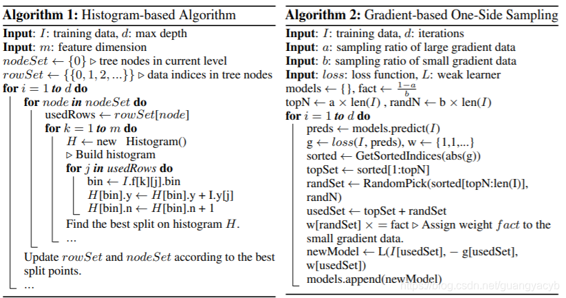
GBDT is an ensemble model of decision trees, which are trained in sequence [1]. In each iteration, GBDT learns the decision trees by fitting the negative gradients (also known as residual errors). The main cost in GBDT lies in learning the decision trees, and the most time-consuming part in learning a decision tree is to find the best split points. One of the most popular algorithms to find split points is the pre-sorted algorithm [8, 9], which enumerates all possible split points on the pre-sorted feature values. This algorithm is simple and can find the optimal split points, however, it is inefficient in both training speed and memory consumption. Another popular algorithm is the histogram-based algorithm [10, 11, 12], as shown in Alg. 13 . Instead of finding the split points on the sorted feature values, histogram-based algorithm buckets continuous feature values into discrete bins and uses these bins to construct feature histograms during training. Since the histogram-based algorithm is more efficient in both memory consumption and training speed, we will develop our work on its basis. As shown in Alg. 1, the histogram-based algorithm finds the best split points based on the feature histograms. It costs O(#data × #feature) for histogram building and O(#bin × #feature) for split point finding. Since #bin is usually much smaller than #data, histogram building will dominate the computational complexity. If we can reduce #data or #feature, we will be able to substantially speed up the training of GBDT

• GBDT 是决策树的集成模型，按一定顺序训练。每次迭代中，GBDT通过拟合负梯度（残差）来学习决策树。

• GBDT 最主要的复杂度在学习决策树上，而学习决策树最耗时的部分在于找到最佳分割点。分割点寻找最佳算法之一是预先排序算法，将所有可能的分割点在预先排好序的特征值上标出，这种算法简单且可以找到最佳分割点，然而在训练速度和内存消耗上都不高效。

• 另一个算法是基于直方图的算法那，相比在排好序的特征值上搜寻，直方图算法将连续特征值划分为多个离散的桶，并在训练中通过这些桶构造直方图。因为此方法在内存消耗和训练速度上相对高效，我们将基于此进展工作。直方图算法那基于特征直方图找到最佳分割点。直方图构建复杂度O(#data × #feature)，分割点搜索复杂度O(#bin × #feature)。因为桶的数量通常远小于 #data，直方图构建占据大部分复杂度。若能减少 #data 或#feature，就可以加速GBDT的训练了。

相关工作

There have been quite a few implementations of GBDT in the literature, including XGBoost [13], pGBRT [14], scikit-learn [15], and gbm in R [16] 4 . Scikit-learn and gbm in R implements the presorted algorithm, and pGBRT implements the histogram-based algorithm. XGBoost supports both the pre-sorted algorithm and histogram-based algorithm. As shown in [13], XGBoost outperforms the other tools. So, we use XGBoost as our baseline in the experiment section. To reduce the size of the training data, a common approach is to down sample the data instances. For example, in [5], data instances are filtered if their weights are smaller than a fixed threshold. SGB [20] uses a random subset to train the weak learners in every iteration. In [6], the sampling ratio are dynamically adjusted in the training progress. However, all these works except SGB [20] are based on AdaBoost [21], and cannot be directly applied to GBDT since there are no native weights for data instances in GBDT. Though SGB can be applied to GBDT, it usually hurts accuracy and thus it is not a desirable choice. Similarly, to reduce the number of features, it is natural to filter weak features [22, 23, 7, 24]. This is usually done by principle component analysis or projection pursuit. However, these approaches highly rely on the assumption that features contain significant redundancy, which might not always be true in practice (features are usually designed with their unique contributions and removing any of them may affect the training accuracy to some degree). The large-scale datasets used in real applications are usually quite sparse. GBDT with the pre-sorted algorithm can reduce the training cost by ignoring the features with zero values [13]. However, GBDT with the histogram-based algorithm does not have efficient sparse optimization solutions. The reason is that the histogram-based algorithm needs to retrieve feature bin values (refer to Alg. 1) for each data instance no matter the feature value is zero or not. It is highly preferred that GBDT with the histogram-based algorithm can effectively leverage such sparse property. To address the limitations of previous works, we propose two new novel techniques called Gradientbased One-Side Sampling (GOSS) and Exclusive Feature Bundling (EFB). More details will be introduced in the next sections.

• 文章中有GBDT的多个实现，包括XGBoost，pGBRT，scikit-learn，R语言的gbm。scikit-learn和gbm 实现的是预先排序算法，pGBRT实现了直方图算法。
• XGBoost 同时支持预先排序和直方图算法。在文献[13]中，XGBoost 表现得比其他方法出色。所以我们的实验选择XGBoost 作为baseline。
• 要减少训练样本数，常用方法是下采样。例如文献【5】中当数据权重小于一个指定阈值就被过滤。SGB【20】在每次迭代占用使用随机的子集来训练弱学习器。【6】采样率动态调整。然而所有的方法除了SGB都是基于adaboost的，不能直接应用于GBDT，因为GBDT的数据实例没有权重。即使SGB可以用于GBDT，它会影响准确率，所以也不是理想的选择。
• 类似的，要减少特征数，自然想到对弱特征进行过滤【22,23,7,24】。通常用主成分分析和投影寻踪。然而这些方法高度依赖一个假设：特征有大量冗余，实际应用中未必满足（特征通常由各自的分布产生，去掉任何一个都可能某种程度上影响训练准确率）。实际应用中的大范围数据集往往很稀疏，预先排序的GBDT可以通过忽略0值的特征来减少训练复杂度【13】。然而直方图GBDT没有有效的稀疏优化方案。因为直方图算法需要为每个数据实例提取特征桶的值，无论特征值是否为0.
• 可以处理好稀疏特征的直方图GBDT 还是首选。为解决以往工作的局限性，我们提出两点创新技术：GOSS 梯度单边采样和互斥特征绑定EFB。更多细节在下一节

 

单边梯度采样

In this section, we propose a novel sampling method for GBDT that can achieve a good balance between reducing the number of data instances and keeping the accuracy for learned decision trees.

• 这一节我们对GBDT提出一个新的方法，在减少样本数和保证学到的决策树的准确率上达到一个不错的平衡。

算法描述

In AdaBoost, the sample weight serves as a good indicator for the importance of data instances. However, in GBDT, there are no native sample weights, and thus the sampling methods proposed for AdaBoost cannot be directly applied. Fortunately, we notice that the gradient for each data instance in GBDT provides us with useful information for data sampling. That is, if an instance is associated with a small gradient, the training error for this instance is small and it is already well-trained. A straightforward idea is to discard those data instances with small gradients. However, the data distribution will be changed by doing so, which will hurt the accuracy of the learned model. To avoid this problem, we propose a new method called Gradient-based One-Side Sampling (GOSS).

GOSS keeps all the instances with large gradients and performs random sampling on the instances with small gradients. In order to compensate the influence to the data distribution, when computing the information gain, GOSS introduces a constant multiplier for the data instances with small gradients (see Alg. 2). Specifically, GOSS firstly sorts the data instances according to the absolute value of their gradients and selects the top a×100% instances. Then it randomly samples b×100% instances from the rest of the data. After that, GOSS amplifies the sampled data with small gradients by a constant when calculating the information gain. By doing so, we put more focus on the under-trained instances without changing the original data distribution by much.

• 在AdaBoost 中，样本权重代表了实例的重要性。然而在GBDT中，没有原始的样本权重，因此adaboost提出的采样方法不能直接应用。幸运的是，我们注意到GBDT中每个实例的梯度给我们提供了很有用的信息用于数据采样：若一个实例具有小梯度，这个实例的训练误差就比较小，说明已经训练的较好了（是因为梯度小说明接近极值么？？）。一个直观的想法是丢弃这些小梯度的样本。然而，这么做会改变数据的分布，影响所学模型的准确度。为了避免这个问题，我们提出了新的方法叫做：单边梯度采样（GOSS）

• GOSS 保留所有大梯度样本，对小梯度样本实例采样随机采样。为了补偿对数据分布的影响，在计算信息增益时，GOSS对小梯度的实例添加了一个常数乘子（是否和随机采样率对应，使得采样后的样本数叠加了乘子后，小梯度样本对信息增益贡献和原来相近？？）GOSS首先依照样本梯度的绝对值对其排序，选择前a×100% 个样本。然后对剩余样本（小梯度）应用b×100%的采样率。然后GOSS在计算信息增益时，对采样后的小梯度样本添加一个倍数 放大。从而对训练好的实例赋予更多的关注，同时不过多改变原数据的分布.

理论分析

GBDT uses decision trees to learn a function from the input space X s to the gradient space G [1]. Suppose that we have a training set with n i.i.d. instances {x1, · · · , xn}, where each xi is a vector with dimension s in space  . In each iteration of gradient boosting, the negative gradients of the loss function with respect to the output of the model are denoted as {g1, · · · , gn}. The decision tree model splits each node at the most informative feature (with the largest information gain). For GBDT, the information gain is usually measured by the variance after splitting, which is defined as below.

• GBDT 使用决策树学习从输入空间X到梯度空间G的函数。假设我们有n个样本训练集{x1, · · · , xn}，每个xi是 空间的s维向量。在梯度提升的每个迭代，损失函数关于模型输出的负梯度标记为： {g1, · · · , gn}。决策树模型将每个节点在最多信息（最大信息增益）的特征上分割。对于GBDT，信息增益通常由分割后的方差衡量，定义如下：

定义3.1

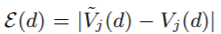
Let O be the training dataset on a fixed node of the decision tree. The variance gain of splitting feature j at point d for this node is defined as

where , and .

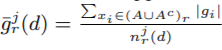
For feature j, the decision tree algorithm selects and calculates the largest gain . 5 Then, the data are split according feature j ∗ at point dj ∗ into the left and right child nodes. In our proposed GOSS method, first, we rank the training instances according to their absolute values of their gradients in the descending order; second, we keep the top-a × 100% instances with the larger gradients and get an instance subset A; then, for the remaining set Ac consisting (1 − a) × 100% instances with smaller gradients, we further randomly sample a subset B with size b × |Ac |; finally, we split the instances according to the estimated variance gain over the subset A ∪ B, i.e.,

where ，，，Br = {xi ∈ B : xij > d}, and the coefficient is used to normalize the sum of the gradients over B back to the size of Ac . Thus, in GOSS, we use the estimated over a smaller instance subset, instead of the accurate over all the instances to determine the split point, and the computation cost can be largely reduced. More importantly, the following theorem indicates that GOSS will not lose much training accuracy and will outperform random sampling. Due to space restrictions, we leave the proof of the theorem to the supplementary materials.

• 让O代表一棵决策树某节点的训练样本，在特征 j 上值为d 处分割的方差增益为：
  
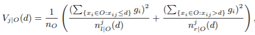
  其中 （该树节点样本数）， （该节点特征j 小于等于d的样本数）， （该节点特征j大于d的样本数）
• 对特征j，决策树算法选择  作为分割点并计算最大增益：，然后数据根据特征  和对应的值  将该节点数据分为左右子节点。
• 在我们提出的GOSS算法中，首先我们将样本按照梯度绝对值降序排列，保留a × 100%个大梯度的实例作为子集A，对于剩余的 (1 − a) × 100%的小梯度子集Ac，我们随机采样出b × |Ac | 大小的子集B，最终我们根据在 A ∪ B上估计的方差增益 来分割样本。
  
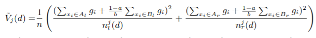
  其中 ，，，Br = {xi ∈ B :xij > d}，系数 是用于将B的梯度和标准化为原来Ac的大小（不是除以b就行么？？）。
• 因此在GOSS中，我们用在子集上估计的，代替在所有样本计算的，来寻找分割点。大大减少了计算复杂度。更重要的是，接下来的理论显示，BOSS不会损失太大的训练准确率，性能比随机采样更好。因为篇幅限制，我们将理论证明放到补充资料中。

理论3.1

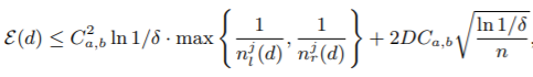
We denote the approximation error in GOSS as and   ， . With probability at least 1 − δ, we have

where , and .

According to the theorem, we have the following discussions: (1) The asymptotic approximation ratio of GOSS is . If the split is not too unbalanced (i.e., and ), the approximation error will be dominated by the second term of Ineq.(2) which decreases to 0 in with n → ∞. That means when number of data is large, the approximation is quite accurate. (2) Random sampling is a special case of GOSS with a = 0. In many cases, GOSS could outperform random sampling, under the condition , which is equivalent to with . Next, we analyze the generalization performance in GOSS. We consider the generalization error in GOSS , which is the gap between the variance gain calculated by the sampled training instances in GOSS and the true variance gain for the underlying distribution. We have . Thus, the generalization error with GOSS will be close to that calculated by using the full data instances if the GOSS approximation is accurate. On the other hand, sampling will increase the diversity of the base learners, which potentially help to improve the generalization performance [24].

• 我们将GOSS中的近似误差记为 ，， ，至少有1 − δ 的概率：
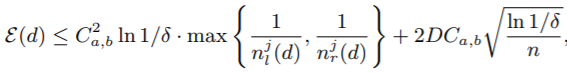  ，其中 ，

• 根据这个理论有以下讨论：

  • GOSS 的渐进近似比为：，若分割很不平衡（且），近似误差会被第二项（2DC……）占据，这一项在n 趋于无穷时根据减小到0。这意味着当数据量很大时，这个近似是较为准确的。

  • 对样本随机采样是GOSS 在a = 0 的一个特殊情况。在多数情况下，GOSS在  下的表现的优于随机采样，这个条件等价于，其中 （结合Ca,b的定义， 等价于） 

• 接下来我们分析GOSS的泛化性能。我们考虑GOSS的泛化误差：，这是GOSS采样过的数据的方差增益和原始数据分布的真实方差增益的误差，有：，因此若GOSS近似是准确的，泛化误差与使用所有数据计算得到的相近。

• 另一方面，采样会增加基础学习器的多样性，潜在改进了泛化性能。

（以上是GOSS方法合理性的说明，详细证明参考相关资料）

 

互斥特征绑定

In this section, we propose a novel method to effectively reduce the number of features

• 本节，我们提出一种新的减少样本特征数的方法。

High-dimensional data are usually very sparse. The sparsity of the feature space provides us a possibility of designing a nearly lossless approach to reduce the number of features. Specifically, in a sparse feature space, many features are mutually exclusive, i.e., they never take nonzero values simultaneously. We can safely bundle exclusive features into a single feature (which we call an exclusive feature bundle). By a carefully designed feature scanning algorithm, we can build the same feature histograms from the feature bundles as those from individual features. In this way, the complexity of histogram building changes from O(#data × #feature) to O(#data × #bundle), while #bundle << #feature. Then we can significantly speed up the training of GBDT without hurting the accuracy. In the following, we will show how to achieve this in detail. There are two issues to be addressed. The first one is to determine which features should be bundled together. The second is how to construct the bundle.

• 高维数据往往很稀疏。特征空间的稀疏性为我们设计一种近似无损的减少特征数方法提供了可能。
• 特别的，在一个稀疏特征空间，很多特征互斥（不会同时取非0值），我们可以安全的将互斥特征绑定为单一特征（成为互斥特征绑定）。通过精心设计一个特征扫描算法，我们可以基于绑定的特征建立与原始独立特征相同的特征直方图。
• 这里直方图构建的构建复杂度从O(#data × #feature) 变为  O(#data × #bundle)，其中 #bundle << #feature。然后可以极大加速GBDT的训练，同时不影响准确率。
• 接下来我们讲述实现细节，有量问题待解决，一个是决定哪些特征要绑定在一起，第二个是如何绑定

理论4.1

The problem of partitioning features into a smallest number of exclusive bundles is NP-hard.

Proof: We will reduce the graph coloring problem [25] to our problem. Since graph coloring problem is NP-hard, we can then deduce our conclusion.

Given any instance G = (V, E) of the graph coloring problem. We construct an instance of our problem as follows. Take each row of the incidence matrix of G as a feature, and get an instance of our problem with |V | features. It is easy to see that an exclusive bundle of features in our problem corresponds to a set of vertices with the same color, and vice versa.

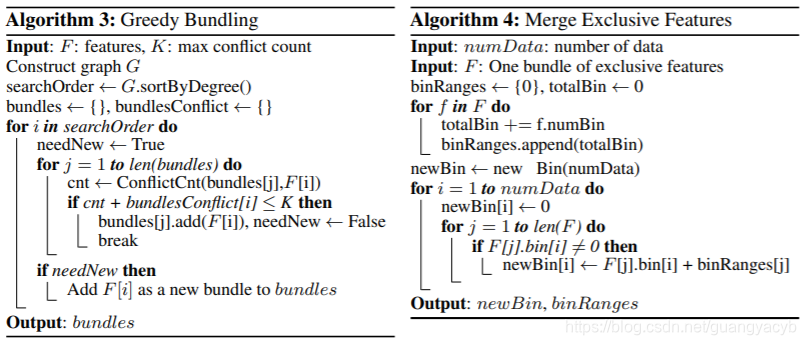
For the first issue, we prove in Theorem 4.1 that it is NP-Hard to find the optimal bundling strategy, which indicates that it is impossible to find an exact solution within polynomial time. In order to find a good approximation algorithm, we first reduce the optimal bundling problem to the graph coloring problem by taking features as vertices and adding edges for every two features if they are not mutually exclusive, then we use a greedy algorithm which can produce reasonably good results (with a constant approximation ratio) for graph coloring to produce the bundles. Furthermore, we notice that there are usually quite a few features, although not 100% mutually exclusive, also rarely take nonzero values simultaneously. If our algorithm can allow a small fraction of conflicts, we can get an even smaller number of feature bundles and further improve the computational efficiency.  By simple calculation, random polluting a small fraction of feature values will affect the training accuracy by at most O([(1 − γ)n] −2/3 )(See Proposition 2.1 in the supplementary materials), where γ is the maximal conflict rate in each bundle. So, if we choose a relatively small γ, we will be able to achieve a good balance between accuracy and efficiency.

Based on the above discussions, we design an algorithm for exclusive feature bundling as shown in Alg. 3. First, we construct a graph with weighted edges, whose weights correspond to the total conflicts between features. Second, we sort the features by their degrees in the graph in the descending order. Finally, we check each feature in the ordered list, and either assign it to an existing bundle with a small conflict (controlled by γ), or create a new bundle. The time complexity of Alg. 3 is O(#feature2 ) and it is processed only once before training. This complexity is acceptable when the number of features is not very large, but may still suffer if there are millions of features. To further improve the efficiency, we propose a more efficient ordering strategy without building the graph: ordering by the count of nonzero values, which is similar to ordering by degrees since more nonzero values usually leads to higher probability of conflicts. Since we only alter the ordering strategies in Alg. 3, the details of the new algorithm are omitted to avoid duplication.

For the second issues, we need a good way of merging the features in the same bundle in order to reduce the corresponding training complexity. The key is to ensure that the values of the original features can be identified from the feature bundles. Since the histogram-based algorithm stores discrete bins instead of continuous values of the features, we can construct a feature bundle by letting exclusive features reside in different bins. This can be done by adding offsets to the original values of the features. For example, suppose we have two features in a feature bundle. Originally, feature A takes value from [0, 10) and feature B takes value [0, 20). We then add an offset of 10 to the values of feature B so that the refined feature takes values from [10, 30). After that, it is safe to merge features A and B, and use a feature bundle with range [0, 30] to replace the original features A and B. The detailed algorithm is shown in Alg. 4.

EFB algorithm can bundle many exclusive features to the much fewer dense features, which can effectively avoid unnecessary computation for zero feature values. Actually, we can also optimize the basic histogram-based algorithm towards ignoring the zero feature values by using a table for each feature to record the data with nonzero values. By scanning the data in this table, the cost of histogram building for a feature will change from O(#data) to O(#non_zero_data). However, this method needs additional memory and computation cost to maintain these per-feature tables in the whole tree growth process. We implement this optimization in LightGBM as a basic function. Note, this optimization does not conflict with EFB since we can still use it when the bundles are sparse

• 将特征分割为最少的互斥捆绑是个NP难题

• 证明：我们引入图上色问题，因为图上色是NP难题，我们可以推导出结论

• 考虑一个上色问题下的图G = (V, E)，我们按照以下步骤构建我们需解决问题的实例。将G的关联矩阵每一行视作特征，那么我们的问题就有|V|个特征。可以看出我们问题里特征的互斥绑定对应于相同颜色的定点集。

• 第一件事（哪些特征绑定在一起），我们证明找到最优绑定策略是NP难题，意味着在多项式时间内找到准确解是不可能的。为了找到一个良好的近似算法，我们先将最优绑定问题简化为图上色问题，其中将特征视作图的定点，若两个特征间不互斥就在对应定点上添加边。然后我们使用贪婪算法（一般可以得到较为合理的不错结果），使用一个近似比常数，用于图上色，以找到绑定关系（相连的定点不能上相同的色，最后相同色的特征顶点可以绑定在一起）。我们注意到很多特征即使不是100%互斥，也极少会在同一特征上取非零值。 若我们的算法允许一小部分冲突，我们可以得到更小的特征绑定集合，进一步提高计算效率。简单计算下，随机污染一小部分特征值会对训练准确率造成最多 的影响（详见补充资料）， γ 是每个绑定中的最大冲突率。所以我们选择一个而相对小的 γ，能够在准确率和效率中达到一个好的平衡。（将特征分成多份绑定，每一份中的特征应互斥，允许的冲突率越大，对互斥的要求越低？）

• 基于以上讨论，我们为互斥特征绑定设计一套算法。首先我们构建一个加权图，权重表示特征之间的冲突（是指同时取非0值的次数？？）。然后我们按照特征（顶点）的度数（出入度）降序排列，接着我们按顺序考察每个特征，要么将其放入一个已有的绑定中（y控制冲突），或创建一个新的绑定。时间复杂度是 O(#feature2 ) ，只需要在训练前处理一次。当特征数不是特别大时，这个复杂度可以接受，但有上百万特征时依然是个问题。为了进一步提高效率，我们提出一个更有效的排序策略（不需构建图）：按照非0值的数量排序，这与按度数排序近似，因为更多的非0值意味着更高的冲突概率（有冲突就是有关联了，在图中就会有边，度数就多了）。因为我们值改变了排序的策略，算法其他细节这里省略。

• 第二个问题（如何绑定），我们需要一个好方法来将同一份绑定中的特征合并，以减少训练复杂度。关键在于保证原特征值可以在绑定中识别出。因为直方图算法存储了离散的桶而不是特征的连续值，我们可以构建一个绑定，使得互斥特征落到不同的桶中。可以通过对特征的原始值添加一个偏移来完成。例如我们再一个绑定中有两个特征，特征A取值范围 [0,10)，特征B取值范围 [0, 20)，我们对特征B添加一个偏移10，调整后的特征取值范围是[10,30)。这样就能安全的合并特征A和B，该特征绑定的取值范围是[0, 30)。

• EFB 算法可以将多个互斥特征绑定，转化为更少的紧密联系的特征，减少了0特征值的不必要计算。实际上我们可以优化基本的直方图算法以忽略0特征值，这要通过使用一个特征表只记录每个特征非0的值。通过扫描这张表，特征的直方图构建复杂度从O(#data) 到O(#non_zero_data)。然而此方法需要额外存储空间还有额外计算，在树增长过程中存放着特征表。我们在LightGBM  将此优化 作为一个基本函数。注意这个优化与EFB不冲突，因为在绑定很稀疏时依然会使用它。

 

实验

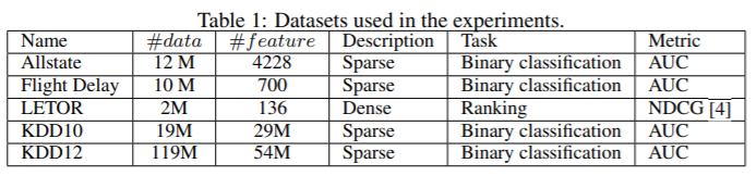
In this section, we report the experimental results regarding our proposed LightGBM algorithm. We use five different datasets which are all publicly available. The details of these datasets are listed in Table 1. Among them, the Microsoft Learning to Rank (LETOR) [26] dataset contains 30K web search queries. The features used in this dataset are mostly dense numerical features. The Allstate Insurance Claim [27] and the Flight Delay [28] datasets both contain a lot of one-hot coding features. And the last two datasets are from KDD CUP 2010 and KDD CUP 2012. We directly use the features used by the winning solution from NTU [29, 30, 31], which contains both dense and sparse features, and these two datasets are very large. These datasets are large, include both sparse and dense features, and cover many real-world tasks. Thus, we can use them to test our algorithm thoroughly. Our experimental environment is a Linux server with two E5-2670 v3 CPUs (in total 24 cores) and 256GB memories. All experiments run with multi-threading and the number of threads is fixed to 16

• 这一节展示我们提出的LightGBM 的实验结果。我们使用5哥不同的公开数据集，数据细节见表1.Microsoft Learning to Rank 数据集有30k个网络查询。这个数据集的特征是稠密的数值特征。Allstate Insurance Claim 和 Flight Delay数据集都包含了很多独热编码特征。最后两个数据集来自 KDD CUP 2010和 KDD CUP 2012.我们直接使用取胜解法的特征，包含了稠密和稀疏的特征。

• 这些数据集都很庞大，包含了稠密与稀疏特征，覆盖了很多实际任务。因此我们用他们来彻底测试下算法。

• 我们实验环境是 linux服务器，两块 E5-2670 v3 CPU，256G内存。所有实验用多线程跑，线程数为16.

整体比较

We present the overall comparisons in this subsection. XGBoost [13] and LightGBM without GOSS and EFB (called lgb_baselline) are used as baselines. For XGBoost, we used two versions, xgb_exa (pre-sorted algorithm) and xgb_his (histogram-based algorithm). For xgb_his, lgb_baseline, and LightGBM, we used the leaf-wise tree growth strategy [32]. For xgb_exa, since it only supports layer-wise growth strategy, we tuned the parameters for xgb_exa to let it grow similar trees like other

• 这里我们列出整体比较。XGBoost 和 不带GOSS和EFB的LightGBM 作为baseline。
• XGBoost 使用两个版本：xgb_exa （预先排序算法）和xgb_his （直方图算法）（查询分割点）
• 对 xgb_his, lgb_baseline, LightGBM 我们使用按叶子的增长策略。
• 对于xgb_exa，因为只支持按层的增长策略，我们调整参数，使得生成的树和其他的类似。

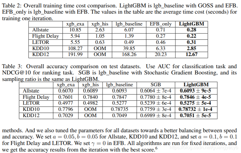
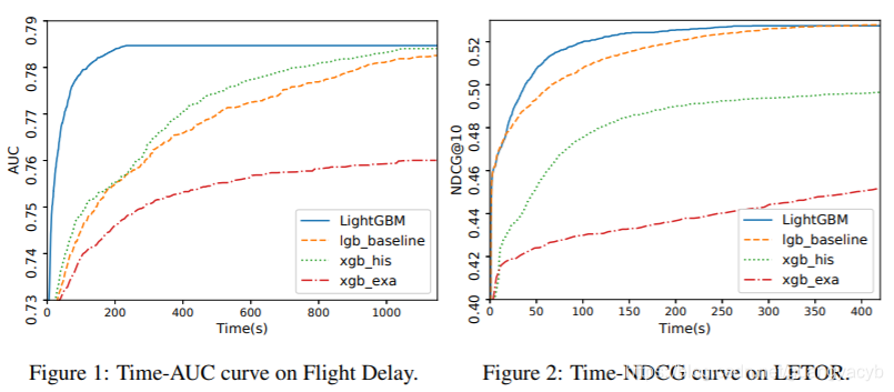
The training time and test accuracy are summarized in Table 2 and Table 3 respectively. From these results, we can see that LightGBM is the fastest while maintaining almost the same accuracy as baselines. The xgb_exa is based on the pre-sorted algorithm, which is quite slow comparing with histogram-base algorithms. By comparing with lgb_baseline, LightGBM speed up 21x, 6x, 1.6x, 14x and 13x respectively on the Allstate, Flight Delay, LETOR, KDD10 and KDD12 datasets. Since xgb_his is quite memory consuming, it cannot run successfully on KDD10 and KDD12 datasets due to out-of-memory. On the remaining datasets, LightGBM are all faster, up to 9x speed-up is achieved on the Allstate dataset. The speed-up is calculated based on training time per iteration since all algorithms converge after similar number of iterations. To demonstrate the overall training process, we also show the training curves based on wall clock time on Flight Delay and LETOR in the Fig. 1

• 训练时间和测试准确度在表2和表3中呈现。
• 从这里结果看，LightGBM是最快的，且达到与baseline几乎相同的准确率。
• xgb_exa 基于预先排序算法那，相对直方图算法太慢
• 与lgb_baseline相比，LightGBM 在Allstate, Flight Delay, LETOR, KDD10 ， KDD12数据集将速度提高了不同倍数：21x, 6x, 1.6x, 14x，13x 
• 因为xgb_his比较消耗内存，无法成功跑KDD10 、 KDD12数据集（因为内存溢出了）
• 在剩余数据集中，LightGBM 都是最快的，速度提高了9倍。因为每个算法在相近的迭代次数后收敛，这里的速度计算基于每次迭代的时间。

and Fig. 2, respectively. To save space, we put the remaining training curves of the other datasets in the supplementary material. On all datasets, LightGBM can achieve almost the same test accuracy as the baselines. This indicates that both GOSS and EFB will not hurt accuracy while bringing significant speed-up. It is consistent with our theoretical analysis in Sec. 3.2 and Sec. 4. LightGBM achieves quite different speed-up ratios on these datasets. The overall speed-up comes from the combination of GOSS and EFB, we will break down the contribution and discuss the effectiveness of GOSS and EFB separately in the next sections.

分析GOSS

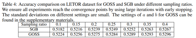
First, we study the speed-up ability of GOSS. From the comparison of LightGBM and EFB_only (LightGBM without GOSS) in Table 2, we can see that GOSS can bring nearly 2x speed-up by its own with using 10% - 20% data. GOSS can learn trees by only using the sampled data. However, it retains some computations on the full dataset, such as conducting the predictions and computing the gradients. Thus, we can find that the overall speed-up is not linearly correlated with the percentage of sampled data. However, the speed-up brought by GOSS is still very significant and the technique is universally applicable to different datasets. Second, we evaluate the accuracy of GOSS by comparing with Stochastic Gradient Boosting (SGB) [20]. Without loss of generality, we use the LETOR dataset for the test. We tune the sampling ratio by choosing different a and b in GOSS, and use the same overall sampling ratio for SGB. We run these settings until convergence by using early stopping. The results are shown in Table 4. We can see the accuracy of GOSS is always better than SGB when using the same sampling ratio. These results are consistent with our discussions in Sec. 3.2. All the experiments demonstrate that GOSS is a more effective sampling method than stochastic sampling.

• 首先我们研究GOSS的加速特性。通过将LightGBM 与EFB_only 比较，我们发现使用10%-20%数据，GOSS可以带来2倍的速度提升。GOSS可以只用采样的数据来学习树模型。然而在完整数据集上，它保留了一些计算例如预测和梯度计算。因此我们发现整体的加速与采样比例不是线性相关。尽管如此，GOSS带来的加速仍然很可观，对于不同数据集都可应用。

• 其次，我们评估GOSS的准确性，通过与随机梯度下降比较。为不是一般性，我们使用LETOR数据集。我们选择GOSS不同的a和b参数，对于SGB使用相同的全局采样比例。在此参数下训练至收敛。结果在表4.可以看出在使用相同采样比率下，总是比SGB好。这个结果与3.2说的一致，所有结果显示GOSS相比随机采样更有效。

分析EFB

We check the contribution of EFB to the speed-up by comparing lgb_baseline with EFB_only. The results are shown in Table 2. Here we do not allow the confliction in the bundle finding process (i.e., γ = 0).7 We find that EFB can help achieve significant speed-up on those large-scale datasets. Please note lgb_baseline has been optimized for the sparse features, and EFB can still speed up the training by a large factor. It is because EFB merges many sparse features (both the one-hot coding features and implicitly exclusive features) into much fewer features. The basic sparse feature optimization is included in the bundling process. However, the EFB does not have the additional cost on maintaining nonzero data table for each feature in the tree learning process. What is more, since many previously isolated features are bundled together, it can increase spatial locality and improve cache hit rate significantly. Therefore, the overall improvement on efficiency is dramatic. With above analysis, EFB is a very effective algorithm to leverage sparse property in the histogram-based algorithm, and it can bring a significant speed-up for GBDT training process.

• 我们核实EFB的加速，通过比较lgb_baseline 与EFB_only。结果在表2.
• 在绑定搜索过程中，我们不允许冲突。发现EFB可以在大规模数据集上达到明显的加速。注意lgb_baseline针对稀疏特征已做优化。而EFB仍然可以极大的对训练过程提速。这是因为EFB合并了很多稀疏特征（包括独热编码特征和互斥特征）。绑定过程中引入了基本的稀疏特征优化。EFB 不需要额外的开销（每个特征的非0值数据表）。因为很多互斥特征绑定在一起，可以提高数据本地化来增加内存命中率。因此，整体效率提升是很可观的。
• 基于以上分析，EFB是直方图算法中处理稀疏特征的有效算法，提速了GBDT的训练过程。

结论

In this paper, we have proposed a novel GBDT algorithm called LightGBM, which contains two novel techniques: Gradient-based One-Side Sampling and Exclusive Feature Bundling to deal with large number of data instances and large number of features respectively. We have performed both theoretical analysis and experimental studies on these two techniques. The experimental results are consistent with the theory and show that with the help of GOSS and EFB, LightGBM can significantly outperform XGBoost and SGB in terms of computational speed and memory consumption. For the future work, we will study the optimal selection of a and b in Gradient-based One-Side Sampling and continue improving the performance of Exclusive Feature Bundling to deal with large number of features no matter they are sparse or not.

• 文本提出了新的GBDT算法 LightGBM，包含两种新技术：单边梯度采样和互斥特征绑定 来解决大规模数据和特征。我们从理论分析和实验研究对其进行验证。实验结果与理论相符，展现了在GOSS和EFB下，LightGBM 可以极大处处XGBoost 和SGB的性能，尤其在计算速度和内存开销上。
• 对于未来的工作，我们将研究GOSS中a和b的最优选择，继续提高EFB在处理大规模特征下的性能，包括稀疏与否。

 

学习小结：

本篇降到了lightgbm很多优化，但是看完感觉有些思路还不太清晰，最好结合一些优秀博客来学习

LightGBM算法总结 对直方图的优化（减少要遍历的值）做了详尽表述 

LightGBM Established: October 1, 2016 官网介绍

Features 官方文档 

快的不要不要的lightGBM 对特征的绑定有讲述