caffe学习:calssfication示例解析

最新推荐文章于 2020-09-03 09:34:42 发布

hukai7190

最新推荐文章于 2020-09-03 09:34:42 发布

阅读量693

点赞数

分类专栏： caffe 文章标签： Caffe

本文链接：https://blog.csdn.net/hanging_gardens/article/details/79064504

版权

caffe 专栏收录该内容

17 篇文章 0 订阅

订阅专栏

结合前面学习的内容,整理一下caffe的官方示例,

Classification: Instant Recognition with Caffe

In this example we’ll classify an image with the bundled CaffeNet model (which is based on the network architecture of Krizhevsky et al. for ImageNet).

We’ll compare CPU and GPU modes and then dig into the model to inspect features and the output.

1. Setup

First, set up Python, numpy, and matplotlib.

# set up Python environment: numpy for numerical routines, and matplotlib for plotting
import numpy as np
import matplotlib.pyplot as plt

# display plots in this notebook
%matplotlib inline#此处是为了能在notebook中直接显示图像

# set display defaults
# rcParams是一个包含各种参数的字典结构，含有多个key-value，可修改其中部分值

#1. 图像显示大小，单位是英寸
plt.rcParams['figure.figsize'] = (10, 10)        # large images

#2. 最近邻差值,像素为正方形
plt.rcParams['image.interpolation'] = 'nearest'  # don't interpolate: show square pixels

#3. 使用灰度输出而不是彩色输出
plt.rcParams['image.cmap'] = 'gray'  # use grayscale output rather than a (potentially misleading) color heatmap

Load caffe.

# The caffe module needs to be on the Python path;
#  we'll add it here explicitly.
import sys
caffe_root = '../'  # this file should be run from {caffe_root}/examples (otherwise change this line)

# sys.path是一个列表，insert()函数插入一行，也可以使用sys.path.append('模块地址')
sys.path.insert(0, caffe_root + 'python')

import caffe
# If you get "No module named _caffe", either you have not built pycaffe or you have the wrong path.

If needed, download the reference model (“CaffeNet”, a variant of AlexNet).

import os
# 如果该路径下存在caffemodel文件，则打印信息，否则从官网下载
if os.path.isfile(caffe_root + 'models/bvlc_reference_caffenet/bvlc_reference_caffenet.caffemodel'):
    print 'CaffeNet found.'
else:
    print 'Downloading pre-trained CaffeNet model...'
    !../scripts/download_model_binary.py ../models/bvlc_reference_caffenet

output:

Downloading pre-trained CaffeNet model…
…1%, 2 MB, 7 KB/s, 384 seconds passeddd^CTraceback (most recent call last):
File “../scripts/download_model_binary.py”, line 74, in
frontmatter[‘caffemodel_url’], model_filename, reporthook)
File “/usr/lib/python2.7/urllib.py”, line 94, in urlretrieve
return _urlopener.retrieve(url, filename, reporthook, data)
File “/usr/lib/python2.7/urllib.py”, line 268, in retrieve
block = fp.read(bs)
File “/usr/lib/python2.7/socket.py”, line 380, in read
data = self._sock.recv(left)
KeyboardInterrupt

2. Load net and set up input preprocessing

Set Caffe to CPU mode and load the net from disk.

caffe.set_mode_cpu()#设置caffe为cpu模式

model_def = caffe_root + 'models/bvlc_reference_caffenet/deploy.prototxt'
model_weights = caffe_root + 'models/bvlc_reference_caffenet/bvlc_reference_caffenet.caffemodel'

#加载model和network
net = caffe.Net(model_def,      # defines the structure of the model #定义模型结构
                model_weights,  # contains the trained weights #包含模型训练权重
                caffe.TEST)     # use test mode (e.g., don't perform dropout) #使用测试模型(如,不使用dropout)

Set up input preprocessing. (We’ll use Caffe’s caffe.io.Transformer to do this, but this step is independent of other parts of Caffe, so any custom preprocessing code may be used).

Our default CaffeNet is configured to take images in BGR format. Values are expected to start in the range [0, 255] and then have the mean ImageNet pixel value subtracted from them. In addition, the channel dimension is expected as the first (outermost) dimension.

As matplotlib will load images with values in the range [0, 1] in RGB format with the channel as the innermost dimension, we are arranging for the needed transformations here.

# load the mean ImageNet image (as distributed with Caffe) for subtraction
# 加载ImageNet训练集的图像均值，预处理需要减去均值
# ilsvrc_2012_mean.npy文件是numpy格式，其数据维度是(3L, 256L, 256L)
mu = np.load(caffe_root + 'python/caffe/imagenet/ilsvrc_2012_mean.npy')

# 对所有像素值取平均以此获取BGR的均值像素值
mu = mu.mean(1).mean(1)  # average over pixels to obtain the mean (BGR) pixel values
print 'mean-subtracted values:', zip('BGR', mu)
# 取平均后得到BGR均值分别是 [('B', 104.0069879317889), ('G', 116.66876761696767), ('R', 122.6789143406786)]

# create transformer for the input called 'data'
# 对输入数据进行变换

# caffe.io.transformer是一个类，实体化的时候构造函数__init__(self, inputs)给一个初值
# 其中net.blobs本身是一个字典，每一个key对应每一层的名字
# 见deploy.prototxt
# net.blobs['data'].data.shape计算结果为(10, 3, 227, 227)
transformer = caffe.io.Transformer({'data': net.blobs['data'].data.shape}) 

# 以下都是caffe.io.transformer类的函数方法
#caffe.io.transformer的类定义放在io.py文件中，也可用help函数查看说明

#改变维度的顺序，由原始图片(227,227,3)变为(3,227,227)
transformer.set_transpose('data', (2,0,1))  # move image channels to outermost dimension

#每个通道减去均值
transformer.set_mean('data', mu)            # subtract the dataset-mean value in each channel 

# 缩放到[0，255]之间
transformer.set_raw_scale('data', 255)      # rescale from [0, 1] to [0, 255]

#交换通道，将图片由RGB变为BGR
transformer.set_channel_swap('data', (2,1,0))  # swap channels from RGB to BGR

output:

mean-subtracted values: [(‘B’, 104.0069879317889), (‘G’, 116.66876761696767), (‘R’, 122.6789143406786)]

3. CPU classification

Now we’re ready to perform classification. Even though we’ll only classify one image, we’ll set a batch size of 50 to demonstrate batching.

# set the size of the input (we can skip this if we're happy
#  with the default; we can also change it later, e.g., for different batch sizes)
net.blobs['data'].reshape(50,        # batch size
                          3,         # 3-channel (BGR) images
                          227, 227)  # image size is 227x227

Load an image (that comes with Caffe) and perform the preprocessing we’ve set up.

image = caffe.io.load_image(caffe_root + 'examples/images/cat.jpg') #加载图片
transformed_image = transformer.preprocess('data', image) # 执行上面设置的图片预处理操作,并将图片载入到blob中
plt.imshow(image)

output:

<matplotlib.image.AxesImage at 0x7f09693a8c90>

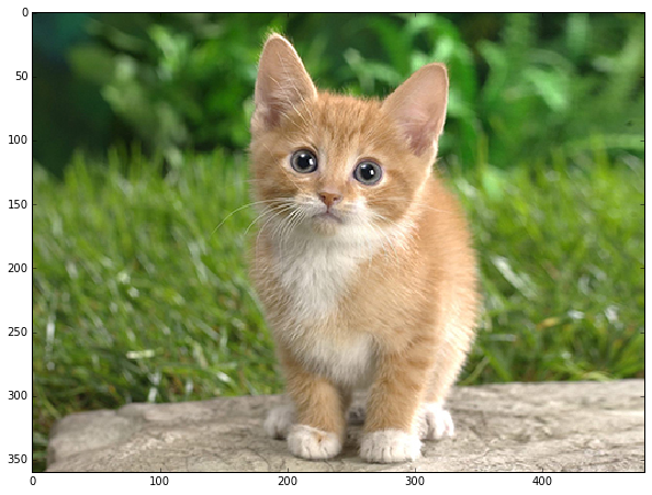
Adorable! Let’s classify it!

# copy the image data into the memory allocated for the net
net.blobs['data'].data[...] = transformed_image

### perform classification
# 前向传播，跑一遍网络，默认结果为最后一层的blob（也可以指定某一中间层），赋给output
output = net.forward()

# output['prob']矩阵的维度是(50, 1000)
# 取batch中第一张图像的概率值
output_prob = output['prob'][0]  # the output probability vector for the first image in the batch

# 打印概率最大的类别代号，argmax()函数是求取矩阵中最大元素的索引
print 'predicted class is:', output_prob.argmax()

predicted class is: 281

The net gives us a vector of probabilities; the most probable class was the 281st one. But is that correct? Let’s check the ImageNet labels…

网络输出是一个概率向量，最可能的类别是第281个类别。但是结果是否正确呢，需要查看一下ImageNet的标签

# load ImageNet labels
# 加载ImageNet标签，如果不存在，则会自动下载
labels_file = caffe_root + 'data/ilsvrc12/synset_words.txt'
if not os.path.exists(labels_file):
    !../data/ilsvrc12/get_ilsvrc_aux.sh

# 读取纯文本数据，三个参数分别是文件地址、数据类型和数据分隔符，保存为字典格式
labels = np.loadtxt(labels_file, str, delimiter='\t')

print 'output label:', labels[output_prob.argmax()]

output label: n02123045 tabby, tabby cat

“Tabby cat” is correct! But let’s also look at other top (but less confident predictions).

# sort top five predictions from softmax output
# 从softmax output可查看置信度最高的五个结果
# 逆序排列，取前五个最大值
top_inds = output_prob.argsort()[::-1][:5]  # reverse sort and take five largest items

print 'probabilities and labels:'
zip(output_prob[top_inds], labels[top_inds])

probabilities and labels:

[(0.31243637, ‘n02123045 tabby, tabby cat’),
(0.2379719, ‘n02123159 tiger cat’),
(0.12387239, ‘n02124075 Egyptian cat’),
(0.10075711, ‘n02119022 red fox, Vulpes vulpes’),
(0.070957087, ‘n02127052 lynx, catamount’)]

We see that less confident predictions are sensible.

4. Switching to GPU mode

Let’s see how long classification took, and compare it to GPU mode.

# 查看CPU的分类时间，然后再与GPU进行比较
%timeit net.forward()#计时

1 loop, best of 3: 1.42 s per loop

That’s a while, even for a batch of 50 images. Let’s switch to GPU mode.

#gpu模式下跑一次
# 使用第一块显卡
caffe.set_device(0)  # if we have multiple GPUs, pick the first one

# 设为gpu模式
caffe.set_mode_gpu()

#前向传播
net.forward()  # run once before timing to set up memory
%timeit net.forward()#计时

10 loops, best of 3: 70.2 ms per loop

That should be much faster!

5. Examining intermediate output

A net is not just a black box; let’s take a look at some of the parameters and intermediate activations.

First we’ll see how to read out the structure of the net in terms of activation and parameter shapes.

For each layer, let’s look at the activation shapes, which typically have the form (batch_size, channel_dim, height, width).

The activations are exposed as an OrderedDict, net.blobs.

卷积神经网络不单单是一个黑盒子。我们接下来看看该模型的一些参数和一些中间输出。首先，我们来看下如何读取网络的结构(每层的名字以及相应层的参数)。

net.blob对应网络每一层数据，对于每一层，都是四个维度：(batch_size, channel_dim, height, width)。

# for each layer, show the output shape
# 循环打印每一层名字和相应维度
for layer_name, blob in net.blobs.iteritems():
    print layer_name + '\t' + str(blob.data.shape)

data (50, 3, 227, 227)
conv1 (50, 96, 55, 55)
pool1 (50, 96, 27, 27)
norm1 (50, 96, 27, 27)
conv2 (50, 256, 27, 27)
pool2 (50, 256, 13, 13)
norm2 (50, 256, 13, 13)
conv3 (50, 384, 13, 13)
conv4 (50, 384, 13, 13)
conv5 (50, 256, 13, 13)
pool5 (50, 256, 6, 6)
fc6 (50, 4096)
fc7 (50, 4096)
fc8 (50, 1000)
prob (50, 1000)

Now look at the parameter shapes. The parameters are exposed as another OrderedDict, net.params. We need to index the resulting values with either [0] for weights or [1] for biases.

The param shapes typically have the form (output_channels, input_channels, filter_height, filter_width) (for the weights) and the 1-dimensional shape (output_channels,) (for the biases).

net.params对应网络中的参数（卷积核参数，全连接层参数等），有两个字典值，net.params[0]是权值（weights），net.params[1]是偏移量（biases），权值参数的维度表示是(output_channels, input_channels, filter_height, filter_width)，偏移量参数的维度表示(output_channels,)

# 循环打印参数名称，权值参数和偏移量参数的维度
for layer_name, param in net.params.iteritems():
    print layer_name + '\t' + str(param[0].data.shape), str(param[1].data.shape)

conv1 (96, 3, 11, 11) (96,)
conv2 (256, 48, 5, 5) (256,)
conv3 (384, 256, 3, 3) (384,)
conv4 (384, 192, 3, 3) (384,)
conv5 (256, 192, 3, 3) (256,)
fc6 (4096, 9216) (4096,)
fc7 (4096, 4096) (4096,)
fc8 (1000, 4096) (1000,)

Since we’re dealing with four-dimensional data here, we’ll define a helper function for visualizing sets of rectangular heatmaps.

#这里要将四维数据进行特征可视化，需要一个定义辅助函数：
def vis_square(data):
    """Take an array of shape (n, height, width) or (n, height, width, 3)
       and visualize each (height, width) thing in a grid of size approx. sqrt(n) by sqrt(n)"""

    # normalize data for display 数据正则化
    data = (data - data.min()) / (data.max() - data.min())

    # force the number of filters to be square
    # 此处目的是将一个个滤波器按照正方形的样子排列
    # 先对shape[0]也就是滤波器数量取平方根，然后取大于等于该结果的正整数
    # 比如40个卷积核，则需要7*7的正方形格子（虽然填不满）
    n = int(np.ceil(np.sqrt(data.shape[0])))
    padding = (((0, n ** 2 - data.shape[0]),
               (0, 1), (0, 1))                 # add some space between filters# 在相邻的卷积核之间加入空白
               + ((0, 0),) * (data.ndim - 3))  # don't pad the last dimension (if there is one)# 不填充最后一维

    # 每张小图片向周围扩展一个白色像素
    data = np.pad(data, padding, mode='constant', constant_values=1)  # pad with ones (white)
    # pad函数声明：pad(array, pad_width, mode, **kwargs)，作用是把list在原维度上进行扩展;
    # pad_width是扩充参数，例如参数((3,2),(2,3));
    # 其中(3，2)为水平方向上，上面加3行，下面加2行；
    # (2，3)为垂直方向上，上面加2行，下面加3行;
    # constant是常数填充的意思。

    # tile the filters into an image
    # 将卷积核平铺成图片
    data = data.reshape((n, n) + data.shape[1:]).transpose((0, 2, 1, 3) + tuple(range(4, data.ndim + 1)))
    data = data.reshape((n * data.shape[1], n * data.shape[3]) + data.shape[4:])

    plt.imshow(data); 
    plt.axis('off')
    plt.show()

First we’ll look at the first layer filters, conv1

# the parameters are a list of [weights, biases]
filters = net.params['conv1'][0].data# 选取conv1的卷积核权值参数
vis_square(filters.transpose(0, 2, 3, 1))# 调用函数显示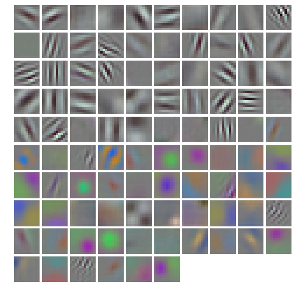

The first layer output, conv1 (rectified responses of the filters above, first 36 only)

feat = net.blobs['conv1'].data[0, :36]
vis_square(feat)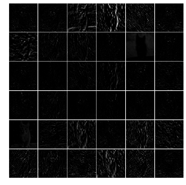

The fifth layer after pooling, pool5

feat = net.blobs['pool5'].data[0]# 选取pool5的第一个输出结果
vis_square(feat)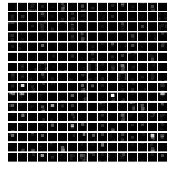

The first fully connected layer, fc6 (rectified)

We show the output values and the histogram of the positive values

feat = net.blobs['fc6'].data[0]# 选取fc6的输出数据，这是一个4096维的向量
plt.subplot(2, 1, 1)
plt.plot(feat.flat)# 平铺向量，图像显示其每一个值
plt.subplot(2, 1, 2)
_ = plt.hist(feat.flat[feat.flat > 0], bins=100)# 做直方图，总共100根条形
plt.show() # 显示两张图表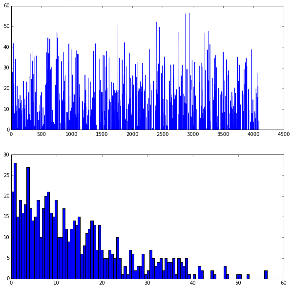

The final probability output, prob

feat = net.blobs['prob'].data[0]# 选取最后一层的输出结果
plt.figure(figsize=(15, 3))# 设置图像大小为（15，3），单位是英寸
plt.plot(feat.flat)# 平铺向量，图像显示其每一个值
plt.show() # 显示图表

[<matplotlib.lines.Line2D at 0x7f09587dfb50>]

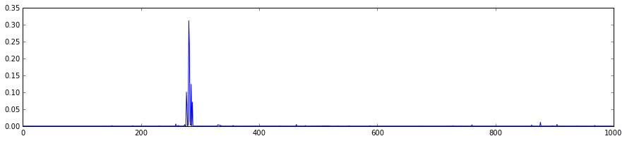
Note the cluster of strong predictions; the labels are sorted semantically. The top peaks correspond to the top predicted labels, as shown above.

6. Try your own image

Now we’ll grab an image from the web and classify it using the steps above.

Try setting my_image_url to any JPEG image URL.

# download an image
my_image_url = "..."  # paste your URL here
# for example:
# my_image_url = "https://upload.wikimedia.org/wikipedia/commons/b/be/Orang_Utan%2C_Semenggok_Forest_Reserve%2C_Sarawak%2C_Borneo%2C_Malaysia.JPG"

# 在线下载图片
!wget -O image.jpg $my_image_url

# transform it and copy it into the net
# 变换图像并将其拷贝到网络
image = caffe.io.load_image('image.jpg')
net.blobs['data'].data[...] = transformer.preprocess('data', image)

# perform classification
# 预测分类结果
net.forward()

# obtain the output probabilities
# 获取输出概率值
output_prob = net.blobs['prob'].data[0]

# sort top five predictions from softmax output
# 将softmax的输出结果按照从大到小排序，并取前5名
top_inds = output_prob.argsort()[::-1][:5]

plt.imshow(image)
plt.show()
print 'probabilities and labels:'
# zip函数依次取值，然后组合
zip(output_prob[top_inds], labels[top_inds])