神经网络的实现

1.numpy

（1）生成numpy数组

# np.arry()接收列表作为参数
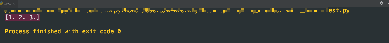
x = np.array([1.0,2.0,3.0])
print(x)

（2）numpy的算数运算

# np.arry()接收列表作为参数
x = np.array([1.0,2.0,3.0])
y = np.array([4.0,5.0,6.0])
# x + y = [5. 7. 9.]
# x + 2 = ..
# x - y = [-3. -3. -3.]
# x - 2 = ..
# x * y = [ 4. 10. 18.] 对应元素(element-wise)相乘
# 2 * x = [2. 4. 6.] 与单一数值(标量)相乘x/y，这个功能也叫广播
# x / y = [0.25 0.4  0.5 ] 对应元素相除
# x / 2 = ..

（3）numpy的多维数组

print("-------一维数组--------")
y = np.array([1,2,3,4])
print(y)
print(np.ndim(y))# 数组的维数
print(y.shape)# 数组的形状
print(y.shape[0])
print("-------二维数组--------")
x = np.array([[1.0,2.0],[3.0,4.0]])
print(x)
print(np.ndim(x))# 数组的维数
print(x.shape)# 数组的形状
print(x.dtype)# 数组元素类型

note：对于数组维数的说明，二维：[[],[],[]]；三维：[[[],[],[]].[[],[],[]]]…

矩阵的运算

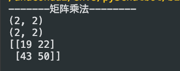
print("-------矩阵乘法--------")
x = np.array([[1, 2], [3, 4]])
y = np.array([[5, 6], [7, 8]])
print(x.shape)
print(y.shape)
print(np.dot(x,y))

数组的算术运算

对应位置进行运算

print("-------数组的算术运算--------")
x = np.array([[1, 2], [3, 4]])
y = np.array([[5, 6], [7, 8]])
print(x + y)
print(x - y)
print(x * y)
print(x / y)

强调一下张量（Tensor）的概念：将一般化之后的向量或矩阵统称为张量。

（4）numpy的广播

# 不同形状的矩阵相乘
x = np.array([[1.0,2.0],[3.0,4.0]])
y = np.array([10,20])
print(10*x)
# 注意此处与数学当中的矩阵相乘不同
print(x*y)

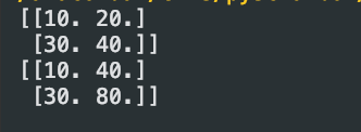此处x*y可以理解成将y扩展成与x同型的数组即[[10,20],[10.20]]然后执行对应位置进行算术运算的操作。

（5）访问元素

x = np.array([[1.0,2.0],[3.0,4.0]])
print(x[0])
print(x[0][0])
for row in x:
    for column  in row:
        print(column)
# 将x转换成一维数组
print(x.flatten())
# 获取索引值为0，3的值
print(x.flatten()[np.array([0,3])])
# 取出小于等于2的值
print(x.flatten()<=2)
print(x.flatten()[x.flatten()<=2])

2.激活函数

阶跃函数

def step_function(x):
    # y是一个bool型的数组，标记x数组中大于小于0的情况
    y = x > 0
    # 将true的位置置1，false的位置置0
    return y.astype(np.int)

sigmod函数

def sigmod(x):
    return 1 / (1 + np.exp(-x))

ReLU函数

def relu(x):
    return np.maximum(0,x)

3.输出层设计

softmax函数

def softmax(a):
    c = np.max(a)
    exp_a = np.(a - c)
    sum_exp_a = np.sum(exp_a)
    y = exp_a / sum_exp_a

    return y

4.损失函数

均方误差

def menn_squared_error(y, t):
    return 0.5 * np.sum((y-t)**2)

交叉熵误差

def cross_entropy_error(y, t):
    delta = 1e-7# 防止log(0)
    return -np.sum(t * np.log(y + delta))
    
# mini_batch版本交叉熵误差的实现,t是用one-hot表示
def cross_entropy_error(y, t):
    if y.ndim == 1:
        t = t.reshape(1, t.size)
        y = y.reshape(1, y.size)
    
    batch_size = y.shape[0]
    return -np.sum(t * np.log(y + 1e-7)) /batch_size
# mini_batch版本交叉熵误差的实现,t非one-hot表示
def cross_entropy_error(y, t):
    if y.ndim == 1:
        t = t.reshape(1, t.size)
        y = y.reshape(1, y.size)

    batch_size = y.shape[0]
    return -np.sum(np.log(y[np.arrange(batch_size), t] + 1e-7)) /batch_size

5、数值微分

利用微小的差分求导的过程称为数值微分，含有误差。
用数学公式求导数过程称为解析性求解或解析性求导，不含误差。

前向差分

def numerical_diff(f, x):
    h = 10e-50
    return (f(x+h) - f(x)) / h

第一处改进：此处h去无限接近0的值，产生了舍入误差(rounding error)，舍入误差就是因省略小数的精细部分的数值而造成最终计算结果上的误差，如：np.float32(1e-50)#结果是0.0无法正确表示出来，此处将h改为1e-04，即10的-4次方就可以得到正确的结果。
第二处改进：上述函数实现的是函数f在x+h和x之间的差分。这个计算一开始就有误差，正确真正的导数是f在x处的斜率，然后这个算式计算的是f在x到x+h处的斜率，这两个是不一致的，原因是h不可能无限接近于0。为了减小这个误差计算f在x+h到x-h之间的差分，此处也叫中心差分。

中心差分

def numerical_diff(f, x):
    h = 1e-4
    return (f(x+h) - f(x-h)) / (2 * h)

画函数图像

# 一维
import numpy as np
import matplotlib.pyplot as plt
# 此处是f(x)=0.01x**2 + 0.1x的图像
def function_1(x):
    return 0.01*x**2 + 0.1*x
    
x = np.arange(0.0, 20.0, 0.1)#0到20，以0.1为单位，将x对应的y值连起来
y = function_1(x)
plt.xlabel("x")
plt.ylabel("f(x)")
plt.plot(x, y)
plt.show()

"""
绘制3d图形
"""

import matplotlib.pyplot as plt
import numpy as np
from mpl_toolkits.mplot3d import Axes3D
# 定义figure
fig = plt.figure()
# 创建3d图形的两种方式
# 将figure变为3d
ax = Axes3D(fig)

#ax = fig.add_subplot(111, projection='3d')

# 定义x, y
x = np.arange(-4, 4, 0.25)
y = np.arange(-4, 4, 0.25)

# 生成网格数据
X, Y = np.meshgrid(x, y)

# 计算每个点对的长度
R = np.sqrt(X ** 2 + Y ** 2)
# 计算Z轴的高度
Z = np.sin(R)


# 绘制3D曲面

# rstride:行之间的跨度(分Y)  cstride:列之间的跨度(分X)
# rcount:设置间隔个数，默认50个，ccount:列的间隔个数  不能与上面两个参数同时出现

# cmap是颜色映射表
# from matplotlib import cm
# ax.plot_surface(X, Y, Z, rstride=1, cstride=1, cmap=cm.coolwarm)
# cmap = "rainbow" 亦可
# 我的理解的 改变cmap参数可以控制三维曲面的颜色组合, 一般我们见到的三维曲面就是 rainbow 的
# 你也可以修改 rainbow 为 coolwarm
ax.plot_surface(X, Y, Z, rstride=1, cstride=1, cmap=plt.get_cmap('rainbow'))

# 绘制从3D曲面到底部的投影,zdir 可选 'z'|'x'|'y'| 分别表示投影到z,x,y平面
# zdir = 'z', offset = -2 表示投影到z = -2上
ax.contour(X, Y, Z, zdir='z', offset=-2, cmap=plt.get_cmap('rainbow'))

# ~ help(ax.plot_surface)
# 设置z轴的维度，x,y类似
ax.set_zlim(-2, 2)

# 设置坐标轴标签
ax.set_xlabel('X label',color='r')
ax.set_ylabel('Y label',color='r')
ax.set_zlabel('Z label',color='r')

#保存 dpi为分辨率, 越大越清楚
# ~ plt.savefig('plot3d_ex.png',dpi=48)

# 绘制三维散点图
# ~ ax.scatter(X[sel, 0], X[sel, 1], X[sel, 2])
plt.show()

偏导数

# 二元函数的定义
def function_2(x):
    #return np.sum(x**2)
    return x[0] + x[1]**2

求x的偏导数偏导数就是固定y，将其看作常数求一元微分。

梯度

# 计算梯度
def numerical_gradient(f, x):
    h = 1e-4
    grad = np.zeros_like(x)# 生成和x形状相同的数组
    for idx in range(x.size):
        tmp_val = x[idx]
        # 计算f(x+h)
        x[idx] = tmp_val + h
        fxh1 = f(x)
        # 计算f(x-h)
        x[idx] = tmp_val - h
        fxh2 = f(x)

        grad[idx] = (fxh1 - fxh2) / (2*h)
        x[idx] = tmp_val# 还原x数组中的值
        
    return grad

# 梯度下降
# f是要进行优化的函数；init_x是初始值；
# lr是学习率，决定在一次学习中应该学习多少，在多大程度上更新参数；
# step_num是梯度法重复的次数，人工设定
def gradient_descent(f, init_x, lr = 0.01, step_num=100):
    x = init_x

    for i in range(step_num):
        grad = numerical_gradient(f, x)
        # x向函数增加最快的方向移动，梯度下降
        x -= lr*grad
    return x# 最优参数

使用这个函数可以计算函数的极小值以及最小值

两层神经网络的实现

class TwoLayerNet:
    # input_size输入层神经元个数，hidden_size隐藏层神经元个数，output_size输出层神经元个数
    def __init__(self, input_size, hidden_size, output_size, weight_init_std=0.01):
        # 初始化权重
        self.params = {}
        # np.random.rand()用高斯分布进行初始化
        self.params['W1'] = weight_init_std * np.random.rand(input_size, hidden_size)
        self.params['b1'] = np.zeros(hidden_size)
        self.params['W2'] = weight_init_std * np.random.rand(hidden_size, output_size)
        self.params['b2'] = np.zeros(output_size)
        
    def predict(self,x):
        W1, W2 = self.params['W1'], self.params['W2']
        b1, b2 = self.params['b1'], self.params['b2']
        
        a1 = np.dot(x, W1) + b1
        z1 = sigmod(a1)
        a2 = np.dot(z1,W2) + b2
        y = softmax(a2)
        
        return y
    
    def loss(self,x , t):
        y = self.predict(x)
        
        return cross_entropy_error(y, t)
    
    def accuracy(self, x, t):
        t = self.predict(x)
        y = np.argmax(y, axis=1)
        t = np.argmax(t, axis=1)
        
        accuracy = np.sum(y == t) /float(x.shape[0])
        return accuracy
    
    def numerical_gradient(self, x, t):
        loss_W = lambda W: self.loss(x, t)
        
        grads = {}
        grads['W1'] = numerical_gradient(loss_W, self.params['W1'])
        grads['b1'] = numerical_gradient(loss_W, self.params['b1'])
        grads['W2'] = numerical_gradient(loss_W, self.params['W2'])
        grads['b2'] = numerical_gradient(loss_W, self.params['b2'])
        
        return grads

mini-batch的实现

# 超参数
iters_num = 10000
train_size = x_train.shape[0]
batch_size = 100
learning_rate = 0.1

train_loss_list = []
train_acc_list = []
test_acc_list = []
# 平均每个epoch的重复次数
iter_per_epoch = max(train_size / batch_size, 1)

network = TwoLayerNet(input_size=784, hidden_size=50, output_size=10)

for i in range(iters_num):
    batch_mask = np.random.choice(train_size,batch_size)
    x_batch = x_train[batch_mask]
    t_batch = x_train[batch_mask]

    # 计算梯度
    grad = network.numerical_gradient(x_batch, t_batch)

    for key in ['W1', 'W2', 'b1', 'b2']:
        network.params[key] -= learning_rate * grad[key]

    # 记录学习过程
    loss = network.loss(x_batch, t_batch)
    train_loss_list.append(loss)
    # 计算每个epoch的识别精度
    if i % iter_per_epoch == 0:
        train_acc = network.accuracy(x_train, t_train)
        test_acc = network.accuracy(x_test, t_test)
        train_acc_list.append(train_acc)
        test_acc_list.append(test_acc)
        
        print("train acc, test acc | " + str(train_acc) + "," + str(test_acc))

6、误差反向传播法

简单层的实现

（1）乘法层

class MulLayer:
    def __init__(self):
        self.x = None
        self.y = None

    def forward(self, x, y):
        self.x = x
        self.y = y
        out = x * y

        return out

    def backward(self, dout):
        # 翻转x和y
        dx = dout * self.y
        dy = dout * self.x

        return dx, dy

（2）加法层

class AddLayer:
    def __init__(self):
        pass
    
    def forward(self, x, y):
        out = x + y
        return out
    
    def backward(self, dout):
    	#将上游的传来的导数(dout)原封不动传递给下游
        dx = dout * 1
        dy = dout * 1
        return dx, dy

激活函数层实现

（1）ReLU层

class Relu:
    def __init__(self):
        self.mask = None

    def forward(self, x):
        # mask数组中小于0的位置改为True
        self.mask = (x <= 0)
        out = x.copy()
        # 将True的位置改为0
        out[self.mask] = 0

        return out

    def backward(self, dout):
        dout[self.mask] = 0
        dx = dout

        return dx

（2）Sigmod层

class Sigmod:
    def __init__(self):
        self.out = None
        
    def forward(self, x):
        out = 1 / (1 + np.exp(-x))
        self.out = out
        
        return out
    
    def backward(self, dout):
        dx = dout * (1.0 - self.out) * self.out
        
        return dx

Affine层实现

class Affine:
    def __init__(self, W, b):
        self.W = W
        self.b = b
        self.x = None
        self.dW = None
        self.db = None
        
    def fowward(self, x):
        self.x = x
        out = np.dot(x, self.W) + self.b
        
        return out
    
    def backward(self, dout):
        dx = np.dot(dout, self.W.T)
        self.dW = np.dot(self.x.T, dout)
        self.db = np.sum(dout, axis = 0)
        
        return dx

Softmax-with-Loss层实现

class SoftmaxWithLoss:
    def __init__(self):
        self.loss = None# 损失
        self.y = None # softmax的输出
        self.t = None # 监督数据(one-hot vector)
        
    def forward(self, x, t):
        self.t = t 
        self.y = softmax(x)
        self.loss = cross_entropy_error(self.y, self.t)
        
        return self.loss
    
    def backward(self, dout = 1):
        batch_size = self.t.shape[0]
        dx = (self.y - self.t) / batch_size
        
        return dx
        

7、与学习相关的技巧

参数的更新

（1）SGD

class SGD:

    """随机梯度下降法（Stochastic Gradient Descent）"""

    def __init__(self, lr=0.01):
        self.lr = lr
        
    def update(self, params, grads):
        for key in params.keys():
            params[key] -= self.lr * grads[key] 

（2）Momentum

class Momentum:

    """Momentum SGD"""

    def __init__(self, lr=0.01, momentum=0.9):
        self.lr = lr
        self.momentum = momentum
        self.v = None
        
    def update(self, params, grads):
        if self.v is None:
            self.v = {}
            for key, val in params.items():                                
                self.v[key] = np.zeros_like(val)
                
        for key in params.keys():
            self.v[key] = self.momentum*self.v[key] - self.lr*grads[key] 
            params[key] += self.v[key]

（3）AdaGrad

class AdaGrad:

    """AdaGrad"""

    def __init__(self, lr=0.01):
        self.lr = lr
        self.h = None
        
    def update(self, params, grads):
        if self.h is None:
            self.h = {}
            for key, val in params.items():
                self.h[key] = np.zeros_like(val)
            
        for key in params.keys():
            self.h[key] += grads[key] * grads[key]
            params[key] -= self.lr * grads[key] / (np.sqrt(self.h[key]) + 1e-7)

（4）Adam

class Adam:

    """Adam (http://arxiv.org/abs/1412.6980v8)"""

    def __init__(self, lr=0.001, beta1=0.9, beta2=0.999):
        self.lr = lr
        self.beta1 = beta1
        self.beta2 = beta2
        self.iter = 0
        self.m = None
        self.v = None
        
    def update(self, params, grads):
        if self.m is None:
            self.m, self.v = {}, {}
            for key, val in params.items():
                self.m[key] = np.zeros_like(val)
                self.v[key] = np.zeros_like(val)
        
        self.iter += 1
        lr_t  = self.lr * np.sqrt(1.0 - self.beta2**self.iter) / (1.0 - self.beta1**self.iter)         
        
        for key in params.keys():
            #self.m[key] = self.beta1*self.m[key] + (1-self.beta1)*grads[key]
            #self.v[key] = self.beta2*self.v[key] + (1-self.beta2)*(grads[key]**2)
            self.m[key] += (1 - self.beta1) * (grads[key] - self.m[key])
            self.v[key] += (1 - self.beta2) * (grads[key]**2 - self.v[key])
            
            params[key] -= lr_t * self.m[key] / (np.sqrt(self.v[key]) + 1e-7)
            
            #unbias_m += (1 - self.beta1) * (grads[key] - self.m[key]) # correct bias
            #unbisa_b += (1 - self.beta2) * (grads[key]*grads[key] - self.v[key]) # correct bias
            #params[key] += self.lr * unbias_m / (np.sqrt(unbisa_b) + 1e-7)

权重的初始值

# coding: utf-8
import numpy as np
import matplotlib.pyplot as plt


def sigmoid(x):
    return 1 / (1 + np.exp(-x))


def ReLU(x):
    return np.maximum(0, x)


def tanh(x):
    return np.tanh(x)
    
input_data = np.random.randn(1000, 100)  # 1000个数据
node_num = 100  # 各隐藏层的节点（神经元）数
hidden_layer_size = 5  # 隐藏层有5层
activations = {}  # 激活值的结果保存在这里

x = input_data

for i in range(hidden_layer_size):
    if i != 0:
        x = activations[i-1]

    # 改变初始值进行实验！
    w = np.random.randn(node_num, node_num) * 1
    # w = np.random.randn(node_num, node_num) * 0.01
    # w = np.random.randn(node_num, node_num) * np.sqrt(1.0 / node_num)
    # w = np.random.randn(node_num, node_num) * np.sqrt(2.0 / node_num)


    a = np.dot(x, w)


    # 将激活函数的种类也改变，来进行实验！
    z = sigmoid(a)
    # z = ReLU(a)
    # z = tanh(a)

    activations[i] = z

# 绘制直方图
for i, a in activations.items():
    plt.subplot(1, len(activations), i+1)
    plt.title(str(i+1) + "-layer")
    if i != 0: plt.yticks([], [])
    # plt.xlim(0.1, 1)
    # plt.ylim(0, 7000)
    plt.hist(a.flatten(), 30, range=(0,1))
plt.show()

Batch Normalization

调整各层的激活值分布使其拥有适当的广度，插入一个对数据分布进行正规化的层

Dropout

class Dropout:
    """
    http://arxiv.org/abs/1207.0580
    """
    def __init__(self, dropout_ratio=0.5):
        self.dropout_ratio = dropout_ratio
        self.mask = None

    def forward(self, x, train_flg=True):
        if train_flg:
            self.mask = np.random.rand(*x.shape) > self.dropout_ratio
            return x * self.mask
        else:
            return x * (1.0 - self.dropout_ratio)

    def backward(self, dout):
        return dout * self.mask