


封面部分
在代码中,显示封面只有一句话
\makecover在文章的开头部分可以编辑封面内容,但我的建议是不用改,因为封面模板经常更新,只需要把学校提供的封面编辑好之后,转换成pdf,再把pdf的内容,替换掉main.pdf(与main.tex同一文件夹,也是代码生成的pdf文件)中相应的内容即可。
封面下载地址:学位管理 - 电子科技大学研究生院
公式部分
在模板中的2.2.1中已经提供了一个公式代码
\begin{equation}
f_n(\bm{r})=
\begin{cases}
\frac{l_n}{2A_n^+}\bm{\rho}_n^+=\frac{l_n}{2A_n^+}(\bm{r}-\bm{r}_+)&\bm{r}\in T_n^+\\
\frac{l_n}{2A_n^-}\bm{\rho}_n^-=\frac{l_n}{2A_n^-}(\bm{r}_--\bm{r})&\bm{r}\in T_n^-\\
0&\text{otherwise}
\end{cases}
\end{equation}
每一个公式的结构都是
\begin{equation}

%公式代码

\end{equation}
或者
\begin{align}

%公式代码

\end{align}利用在线编辑工具:在线LaTeX公式编辑器-编辑器
可以进行编辑,插入相应的符号会自动生成,具体内容自己摸索
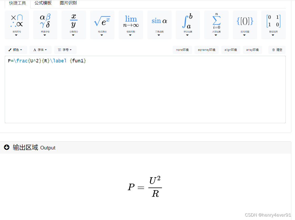
图中的\lable{fun1}是给公式加的标签,正文中添加\ref{fun1}则会生成对公式的引用
latex对公式引用代码,正文中的符号需要加$$符号才可以与公式中的形式一致
根据式(\ref{fun1})可以计算出设备在运行时的功耗数据$P$,式(\ref{fun1})中,$U$为此时的运行电压,$R$为采样电阻,$P$为采样电阻的功耗。
\begin{align}
	P=\frac{U^2}{R}\label{fun1}
\end{align}
多公式,等号对齐的形式,用&符号对齐相应部分,case代码是加大括号
\begin{equation}%公式开始
f_n(\bm{r})=

\begin{cases}%大括号开始

\frac{l_n}{2A_n^+}\bm{\rho}_n^+=\frac{l_n}{2A_n^+}(\bm{r}-\bm{r}_+)&\bm{r}\in T_n^+\\

%      \\是换行符号,多公式的&符号用于不同行的对齐

\frac{l_n}{2A_n^-}\bm{\rho}_n^-=\frac{l_n}{2A_n^-}(\bm{r}_--\bm{r})&\bm{r}\in T_n^-\\

0&\text{otherwise}

\end{cases}%大括号结束


\end{equation}%公式结束
图部分
1、插入简单图
直接把图形文件放到工程的pic文件夹中,然后用代码来显示图,例如放入1.png文件,那么代码为
设备如图\ref{fig1}所示。 %文中对图的引用,这样即使插入新图,标签也不会乱

\begin{figure}[ht] %ht表示当前位置顶部
	\centering
	\includegraphics[width=9cm,height=5.6cm]{1.png} %图片的大小为宽9cm,高5.6cm,参数可调整
	\caption{图的标题}
	\label{fig1}     %定义文内引用的标签
\end{figure}
2、多图显示
多图显示的方法有很多,在这我提供一种1行两列的模板
\begin{figure}[ht]
	\centering
	\begin{minipage}[t]{0.48\textwidth} %占据页面的0.48倍宽度
		\centering
		\includegraphics[width=7.5cm,height=6cm]{1.jpg}
        \subcaption{小标题1}\label{fig1}
	\end{minipage}
	\begin{minipage}[t]{0.48\textwidth} %占据页面的0.48倍宽度
		\centering
		\includegraphics[width=7.5cm,height=6cm]{2.png}
		\subcaption{小标题2}\label{fig2}
	\end{minipage}
    \caption{大标题}
\end{figure}
代码应该还是比较易懂的,读者可通过改变参数调整显示大小(A4纸宽度为15cm)
latex代码作图
插入的图片往往会出现不清晰,字体大小不对的情况,因为图片是引用来的,字体当然会随图片的放大缩小而改变,latex提供tikz模块(代码开始添加),后续我还使用了各种各样的库,可以一次性添加
\usepackage{tikz}
\usepackage{makecell}
\usetikzlibrary{decorations.pathreplacing}
\usetikzlibrary{shapes.geometric}
\usetikzlibrary{shapes, arrows.meta, positioning}
\usetikzlibrary {matrix}
\usepackage{pgfplotstable}
\usepackage{pgfplots}
\pgfplotsset{compat=1.17}
\usepackage{cellspace,tabularx}
\usepackage{array}
\addparagraphcolumntypes{X} % 如果使用tabularx
\usetikzlibrary {circuits.ee.IEC}
可以直接在latex作图,显示出的图片是绝对清晰的,字体大小也是严格正确的,下面提供几种经典类型的作图代码
1、数据流线图
\begin{figure}[ht]
	\begin{tikzpicture}
		{\fontsize{10.5}{14}\selectfont    %图片中的文字大小设为10.5pt,也就是5号字
		\begin{axis}[
			xlabel={横轴标签},
			ylabel={纵轴标签},
			xmin=5, xmax=50,               %横轴的起始结束位置
			ymin=0, ymax=100,              %纵轴的起始结束位置
			xtick={5,10,15,20,25,30,35,40,45,50}, %横轴刻度
			ytick={0,20,40,60,80,100},            %纵轴刻度
			width=8cm,                            % 图片宽度为8厘米
			height=5cm,                           % 图片高度为5厘米
			scale only axis,                      % 文字不随图片放大缩小
			legend pos=south east,                % 样本示例显示在东南角(右下角)
			ymajorgrids=true,
			grid style=dashed,                    % 经纬度显示为虚线
			line width=1pt,                       % 线的宽度为1pt
			]

			% 第一类
			\addplot[color=blue,mark=none,smooth]  %显示为蓝线,不标记点,流线型
			coordinates {
				(5,24)(10,62)(15,89)(20,94)(25,98)(30,99)(35,99)(40,99)(45,99)(50,99)
			};                                     %这里是画点的位置,会用流线串起来
			\addlegendentry{第一类}

			% 第二类
			\addplot[color=purple,mark=none,smooth]
			coordinates {
				(5,31)(10,69)(15,91)(20,93)(25,99)(30,99)(35,99)(40,99)(45,99)(50,99)
			};
			\addlegendentry{第二类}

			% 第三类
			\addplot[color=green,mark=none,smooth]
			coordinates {
				(5,33)(10,75)(15,92)(20,94)(25,99)(30,99)(35,99)(40,99)(45,99)(50,99)
			};
			\addlegendentry{第三类}

			% 第四类
			\addplot[color=red,mark=none,smooth]
			coordinates {
				(5,0)(10,0)(15,0)(20,0)(25,4)(30,11)(35,25)(40,53)(45,70)(50,81)
			};
			\addlegendentry{第四类}


		\end{axis}
	}
	\end{tikzpicture}
    \caption{图标题}
    \label{fig3}  %图标签
\end{figure}
2、代码流程图
\begin{figure}[ht]
	\begin{tikzpicture}[
		% Styles
		inner sep=0pt,
		layer/.style={draw, very thick, rectangle, minimum height=0.5cm, minimum width=2cm},
		line/.style={-latex,very thick,line width =1pt},
		rec/.style={draw, very thick, rectangle, minimum height=0.5cm, minimum width=2cm,rounded corners=10},
		label/.style={densely dashed},
		test/.style={diamond,aspect=2,draw,very thick},
		para/.style={
			trapezium,
			trapezium left angle=70, trapezium right angle=110,
			minimum width=2cm,
			draw,
			very thick,
			text centered,
			text width=1.5cm
		}
		]
		{\fontsize{10.5}{14}\selectfont
			\node[rec,align=center, minimum height=1cm,minimum width=3cm] (raw) at (-4,11) {开始};
			\node[rec,align=center, minimum height=1.5cm,minimum width=4cm] (raw1) at (-4,9) {初始化、启用外部中断 \\ 当前设为无状态};
			\node[rec,align=center, minimum height=1cm,minimum width=3cm] (raw2) at (-4,7) {等待中断};

			\node[test,align=center, minimum height=1cm,minimum width=1cm] (raw4) at (-4,1.5) {当前是否无状态};

			\node[test,align=center, minimum height=1cm,minimum width=1cm] (raw16) at (-4,-1.2) {接收密钥状态};
			\node[para,align=center, minimum height=1cm,minimum width=3cm] (raw5) at (-4,-4) {Rx\_data存入密钥};
			\node[test,align=center, minimum height=1cm,minimum width=1cm] (raw6) at (-7.6,0) {Rx\_data='k'};
			\node[rec,align=center, minimum height=1cm,minimum width=2.5cm] (raw7) at (-9.5,-2) {状态设为\\接收密钥状态};


			\node[test,align=center, minimum height=1cm,minimum width=1cm] (raw8) at
			(-7.6,-4) {Rx\_data='p'};
			\node[rec,align=center,minimum height=1cm,minimum width=2.5cm] (raw9) at (-9.5,-6) {状态设为\\接收明文};
			\node[para,align=center, minimum height=1cm,minimum width=1cm] (raw10) at (-0.5,-1.2) {Rx\_data存入明文};

			\node[test,align=center, minimum height=1cm,minimum width=1cm] (raw18) at (-0.5,-3.5) {明文已收完};


			\node[rec,align=center, minimum height=2cm,minimum width=3cm] (raw12) at (-0.5,-6.5) {加密、发送密文\\ 状态设为0 \\ 清空缓存};
			\node[rec,align=center, minimum height=2cm,minimum width=3cm] (raw3) at (-4,4.5) {收到数据 \\ 触发中断 \\ 数据放入Rx\_data};
			\node[rec,align=center, minimum height=1cm,minimum width=3cm] (raw11) at (-4,-9.1) {结束};
			\node[test,align=center, minimum height=1cm,minimum width=1cm] (raw14) at (-4,-6) {密钥已收完};


			\draw[line] (raw)--(raw1);
			\draw[line] (raw1)--(raw2);
			\draw[line] (raw2)--(raw3);
			\draw[line] (raw3)--(raw4);
			\draw (raw14)--(-6,-6)--(-6,-8)--(-7.4,-8) node[midway, above] {\textcolor{black}{否}};
			\draw[thick, bend right=90] (-7.4,-8) to (-7.8,-8);
			\draw[line] (-7.8,-8)--(-9.5,-8);
			\draw[line] (raw4)--(-7.6,1.5)--(raw6) node[midway, right] {\textcolor{black}{是}};
			\draw[line] (raw16)--(raw10) node[midway, above] {\textcolor{black}{否}};;
			\draw[line] (raw4)--(raw16) node[midway, right] {\textcolor{black}{否}};;
			\draw[line] (raw16)--(raw5) node[midway, right] {\textcolor{black}{是}};;
			\draw[line] (raw6)--(-9.5,0)--(raw7) node[midway, right] {\textcolor{black}{是}};;

			\draw[line] (raw6)--(raw8) node[midway, right] {\textcolor{black}{否}};;

			\draw[line] (raw8)--(-9.5,-4)--(raw9) node[midway, right] {\textcolor{black}{是}};
			\draw[line] (raw8)--(-7.6,-9.1)--(raw11) node[midway, above] {\textcolor{black}{否}};
			\draw[line] (raw9)--(-9.5,-8)--(-11,-8)--(-11,7)--(raw2);
			\draw[line] (raw7)--(-9.5,-3.5)--(-11,-3.5);

			\draw[line] (raw5)--(raw14);

			\draw[line] (raw10)--(raw18);
			\draw[line] (raw18)--(raw12) node[midway, left] {\textcolor{black}{是}};
			\draw[line] (raw12)--(-0.5,-9.1)--(raw11);

			\draw[line] (raw14)--(raw11) node[midway, right] {\textcolor{black}{是}};;
			\draw[line] (raw18)--(1,-3.5)--(1,7)--(raw2) node[midway, above] {\textcolor{black}{否}};
			%\draw[bend left] (A) to (C);
		}
	\end{tikzpicture}
	\caption{代码流程图}
	\label{fig2}
\end{figure}
代码虽然很长,但很好理解,无非就是定义类型,画模块用at标明位置,再用line把不同的模块连接起来
3、简单结构图
\begin{figure}[ht]%
	\begin{tikzpicture}[
		layer/.style={draw, very thin, rectangle, minimum height=1cm, minimum width=2cm}
		]
        {\fontsize{10.5}{14}\selectfont
		\node (vcc) at (0,0) {VCC};
		\node [layer, right of=vcc, node distance=3cm] (R) {采样电阻};

		\node [layer, right of=R, node distance=4cm] (chip) {芯片};

		\node [right of=chip, node distance=4cm] (gnd) {GND};

		\draw (vcc)--(R);
		\draw (R)--(chip);
		\draw (chip)--(gnd);

		\draw (1.5,0)--(1.5,2.5)--(6,2.5);
		\draw (5,0)--(5,2)--(6,2);

		\node[layer,align=center,align=center] (adc) at (9,2.25) {ADC};
		\node (data) at (12,2.25) {采样数据};

		\draw (7,2.25)--(6,3)--(6,1.5)--(7,2.25)--(adc);

		\draw [-latex] (adc)--(data);
	    }
	\end{tikzpicture}
	\caption{电路图}
	\label{fig2}
\end{figure}
4、柱状图
\begin{figure}[ht]
	\begin{tikzpicture}
		{\fontsize{10.5}{14}\selectfont
		\begin{axis}[
			xlabel={训练集数量},
			ylabel={分类成功率(\%)},
			ybar,
			xmin=0, xmax=22000,
			ymin=75, ymax=101,
			xtick={2000,5000,8000,11000,14000,17000,20000},
			ytick={75,80,85,90,95,100},
			width=10cm,    % 图片的宽
			height=6cm,
			scale only axis,
			legend pos=north west,
			ymajorgrids=true,
			grid style=dashed,
			line width=1pt,
			bar width=8pt,
			x tick label style={/pgf/number format/fixed}, % 固定格式,不使用科学计数法
			y tick label style={/pgf/number format/fixed},
			scaled ticks=false
			]

			% SVM

			\addplot[fill=orange,draw=none] coordinates {
				(2000,78)(5000,80)(8000,84)(11000,86)(14000,89)(17000,91)(20000,93)
			};
			\addlegendentry{MLP}

			\addplot[fill=cyan,draw=none] coordinates {
				(2000,80)(5000,83)(8000,92)(11000,98)(14000,98)(17000,99)(20000,99)
			};
			\addlegendentry{CNN}

			\addplot[fill=green,draw=none] coordinates {
				(2000,80)(5000,88)(8000,93)(11000,97)(14000,99)(17000,100)(20000,100)
			};
			\addlegendentry{LSTM}
		\end{axis}
	}
	\end{tikzpicture}
	\caption{标题}
	\label{fig3}
\end{figure}
这个代码也很好看懂,懂英文的应该都懂怎么调整参数
5、大数据图
以上的图都是少量数据,可以手打,但有些图涉及到大量的数据,例如有几万个样本点,这样就需要把样本数据保存在.csv文件中,再调用csv文件来画图,新建一个sot.csv,第一列为横轴,第二列为纵轴,第三列为另一类的纵轴
\begin{figure}[ht]%
	\begin{tikzpicture}
		{\fontsize{10.5}{14}\selectfont
			\begin{axis}[
				xlabel={采样点},
				ylabel={数值},
				width=8cm,    % 设置宽
				height=4.5cm,
				scale only axis,
				x tick label style={/pgf/number format/fixed}, % 固定格式,不使用科学计数法
				y tick label style={/pgf/number format/fixed},
				scaled ticks=false
				]
				% 导入数据并绘制
				\addplot+[
				mark=*,
				mark size=0.3pt, % 调整标记的大小
				mark options={fill=blue}, % 调整标记的颜色
				color=blue, % 线的颜色
				line width=0.5pt % 线的宽度
				] table [col sep=comma, x index=0, y index=1] {sot.csv}; %第0列为横轴,第1列为纵轴
				\addlegendentry{$X_1$}

				\addplot+[
				mark=*,
				mark size=0.3pt, % 调整标记的大小
				mark options={fill=red}, % 调整标记的颜色
				color=red, % 线的颜色
				line width=0.5pt % 线的宽度
				] table [col sep=comma, x index=0, y index=2] {sot.csv};%第0列为横轴,第2列为纵轴
				\addlegendentry{$X_2$}
			\end{axis}
		}
	\end{tikzpicture}
	\caption{标题}
	\label{fig4}
\end{figure}
当然,如果数据量很大,latex执行起来会花很长时间,每次都会,导致后续的编辑工作总是需要等待,这种情况应该把导入数据并绘制的代码删除,保存到其他地方,只画空图,需要显示的时候再放回去。
图片的形式还有很多种,三维图、饼状图、散点图之类的,chatgpt可以给出很多模板,作者就是在chatgpt给的tikz模板基础上进行画图的
表
现在的文章一般要求三线表,只有横线没有竖线,也涉及到多个空格合并的问题,下面给出两个画表模板
1、不涉及合并的模板
\begin{table}[ht]
	\centering % 表格居中
	\caption{标题} \label{tab1}            %定义标题和引用标签
	{\fontsize{10.5}{14}\selectfont        %表中字体大小设为10.5pt,即5号字
	\renewcommand{\arraystretch}{1.3}	   %表格行间距为1.3倍,大约为0.6cm,可以调整
	\begin{tabular}{ *{8}{c} }             %8列的数据

		\toprule[1.5pt]                    %表格头线为1.5pt
		类型    & 1  & 2   & 3   & 4   & 5   & 6   & 7   \\ %\\用于换行,&用于对齐
		\midrule[1.5pt]                    %标题底线为1.5pt
		成功率1 & \ \ 4\% & 11\% & 25\% & 40\% & 66\% & 81\% & 90\% \\
        成功率2 & \ \ 4\% & 11\% & 25\% & 40\% & 66\% & 81\% & 90\% \\
		\bottomrule[1.5pt]                 %表格底线为1.5pt
	\end{tabular}
    }
\end{table}
2、涉及合并的模板
\begin{table}[ht]
	\centering
	\caption{标题}\label{tab3}
	{\fontsize{10.5}{14}\selectfont
		\renewcommand{\arraystretch}{1.3}
		\begin{tabular}{ ccccccc }  % 7列的数据
			\toprule[1.5pt]
			\multirow{2}{*}[-0.3ex]{文\ 本} & \multirow{2}{*}[-0.3ex]{数据信息} & \multirow{2}{*}[-0.3ex]{训练时间} & \multicolumn{4}{c}{\raisebox{0.3ex}[0pt][0pt]{成功率\ /\ 数据量}} \\ \cline{4-7}
			& & & 10 & 25 & 40 & 55 \\
			\midrule[1.5pt]
			方法1 & 不需要 & 不需要 & 0\% & 4\% & 40\% & 92\% \\
			\hline
			方法2 & 需要 & 1000s & 55\% & 95\% & 99\% & 100\% \\
			\bottomrule[1.5pt]
		\end{tabular}
	}
\end{table}
代码中\multirow{2}{*}[-0.3ex]{文\ 本},代表在列方向上合并两个单元格,文本位置下移0.3ex,写入的内容为{文\ 本}
\multicolumn{4}{c}{\raisebox{0.3ex}[0pt][0pt]{成功率\ /\ 数据量}} \\ \cline{4-7},代表行方向上合并4个单元格,单元格位置上升0.3ex(用来调整位置,可以是负数),\cline{4-7}代表在4-7位置上添加下框线
3、多行多列合并
不推荐使用这种形式,排版会很混乱,有兴趣的读者可以自行研究
参考文献部分
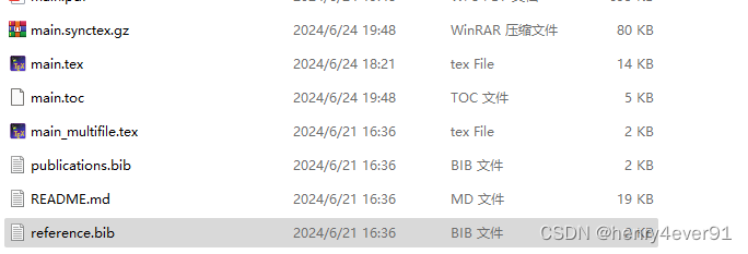
在工程中有个文件reference.bib,用于存储参考文献的内容,publication.bib是用于存储读研期间取得的成果,使用方法差不多
在texstudio中打开 reference.bib文件
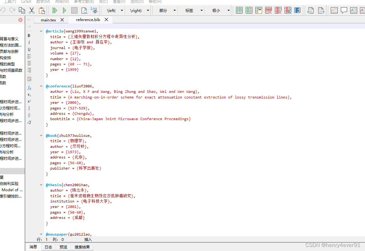
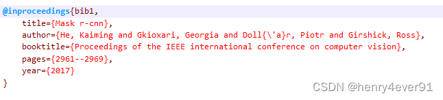
这些都是bibtex类型的代码,google学术上的文章都会提供引用代码
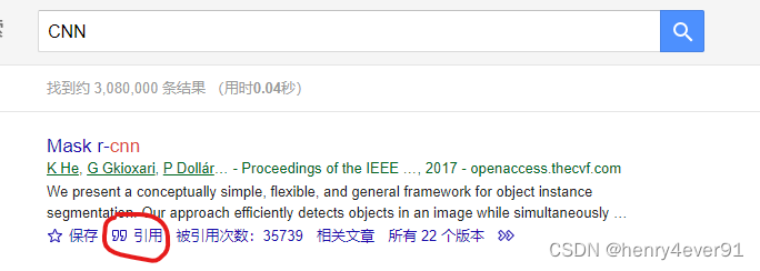
点击引用
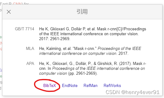

这段代码复制到 reference.bib中把标签改为bib1,保存文件
在文中相应位置写\citing{bib1}就可以显示引用了,当然,在运行代码之前还需要在当前目录中执行下段命令行代码(上一篇文章提到过),否则会出现乱码
xelatex main.tex
bibtex main.aux
bibtex accomplish.aux
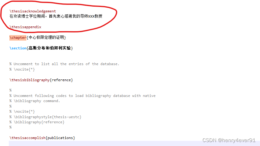
xelatex main.tex成果部分用的publication.bib文件,使用方式也是同理。
致谢和附录写在代码中的相应位置


 289
289

 被折叠的 条评论
为什么被折叠?
被折叠的 条评论
为什么被折叠?
 到【灌水乐园】发言


