图像分割练习

最新推荐文章于 2023-12-27 18:01:43 发布

hesays

最新推荐文章于 2023-12-27 18:01:43 发布

阅读量1.9k

点赞数

分类专栏：数字图像处理文章标签： Matlab 图像处理

数字图像处理专栏收录该内容

8 篇文章 0 订阅

订阅专栏

<h1 class="postTitle" style="margin-bottom: 10px;"><pre name="code" class="html"><h1 class="postTitle" style="margin-bottom: 10px;"><pre name="code" class="html"><h1 class="postTitle" style="margin-bottom: 10px;"><pre name="code" class="html" style="font-weight: bold;"><h1 class="postTitle" style="margin-bottom: 10px;"><span style="font-family:Microsoft YaHei;font-size:14px;"><a target=_blank id="cb_post_title_url" class="postTitle2" href="http://www.cnblogs.com/tornadomeet/archive/2012/03/26/2417555.html">Matlab DIP(瓦)ch10图像分割练习</a></span></h1><h1 class="postTitle" style="margin-bottom: 10px;"><span style="font-family: 'Microsoft YaHei';font-size:14px;">    这一章中主要是用数字图像处理技术对图像进行分割。因为图像分割是个比较难的课题。这里练习的是比较基本的。包过点、线和边缘的检测，hough变换的应用，阈值处理，基于区域的分割以及基于分水岭方法的分割。</span></h1><h1 class="postTitle" style="margin-bottom: 10px;"><pre name="code" class="html"><div id="cnblogs_post_body" style="margin-bottom: 20px;"><p style="margin: 10px auto;"><span style="font-family:Microsoft YaHei;font-size:14px;">   其练习代码和结果如下：</span></p><p style="margin: 10px auto;"><span style="font-family: 'Microsoft YaHei';font-size:14px;">%% 点检测</span></p><p style="margin: 10px auto;"><span style="font-family: Arial, Helvetica, sans-serif; font-size: 12px;">clc</span></p></div>

clear
f=imread('.\images\dipum_images_ch10\Fig1002(a)(test_pattern_with_single_pixel).tif');
subplot(121),imshow(f),title('点检测原图');


w=[-1,-1,-1;
   -1,8,-1;
   -1,-1,-1]
g=abs(imfilter(double(f),w));
subplot(122),imshow(g),title('点检测结果');
%点检测图结果如下：

<img src="https://img-blog.csdn.net/20141215151717950?watermark/2/text/aHR0cDovL2Jsb2cuY3Nkbi5uZXQvaGVzYXlz/font/5a6L5L2T/fontsize/400/fill/I0JBQkFCMA==/dissolve/70/gravity/Center" alt="" />
%% 非线性滤波点检测
clc
clear
f=imread('.\images\dipum_images_ch10\Fig1002(a)(test_pattern_with_single_pixel).tif');
subplot(121),imshow(f),title('非线性滤波点检测原图');


m=3;
n=3;
%ordfilt2(f,order,domin)表示的是用矩阵domin中为1的地方进行排序，然后选择地order个位置的值代替f中的值，属于非线性滤波
g=imsubtract(ordfilt2(f,m*n,ones(m,n)),ordfilt2(f,1,ones(m,n)));%滤波邻域的最大值减去最小值
T=max(g(:));
g2=g>=T;
subplot(122),imshow(g2);
title('非线性滤波点检测后图');
 %运行结果如下：
<img src="https://img-blog.csdn.net/20141215151709062?watermark/2/text/aHR0cDovL2Jsb2cuY3Nkbi5uZXQvaGVzYXlz/font/5a6L5L2T/fontsize/400/fill/I0JBQkFCMA==/dissolve/70/gravity/Center" alt="" />

%% 检测指定方向的线
clc
clear
f=imread('.\images\dipum_images_ch10\Fig1004(a)(wirebond_mask).tif');
subplot(321),imshow(f);
title('检测指定方向线的原始图像');


w=[2 -1 -1;
   -1 2 -1;
   -1 -1 2];%矩阵用逗号或者空格隔开的效果是一样的
g=imfilter(double(f),w);
subplot(322),imshow(g,[]);
title('使用-45度检测器处理后的图像');


gtop=g(1:120,1:120);%取g的左上角图
gtop=pixeldup(gtop,4);%扩大4*4倍的图
subplot(323),imshow(gtop,[]);
title('-45度检测后左上角放大图');


gbot=g(end-119:end,end-119:end);%取右下角图
gbot=pixeldup(gbot,4);%扩大16倍的图
subplot(324),imshow(gbot,[]);
title('-45度检测后右下角后放大图');


g=abs(g);
subplot(325),imshow(g,[]);
title('-45度检测后的绝对值图');


T=max(g(:));
g=g>=T;
subplot(326),imshow(g);
title('-45度检测后取绝对值最大的图')
 64%检测指定方向的线过程如下：
<img src="https://img-blog.csdn.net/20141215151730484?watermark/2/text/aHR0cDovL2Jsb2cuY3Nkbi5uZXQvaGVzYXlz/font/5a6L5L2T/fontsize/400/fill/I0JBQkFCMA==/dissolve/70/gravity/Center" alt="" />

%% sobel检测器检测边缘
clc
clear
f=imread('.\images\dipum_images_ch10\Fig1006(a)(building).tif');
subplot(321),imshow(f);
title('sobel检测的原始图像');


[gv,t]=edge(f,'sobel','vertical');%斜线因为具有垂直分量，所以也能够被检测出来
subplot(322),imshow(gv);
title('sobel垂直方向检测后图像');


gv=edge(f,'sobel',0.15,'vertical');
subplot(323),imshow(gv);
title('sobel垂直检测0.15阈值后图像');


gboth=edge(f,'sobel',0.15);
subplot(324),imshow(gboth);
title('sobel水平垂直方向阈值0.15后图像');


w45=[-2 -1  0
     -1  0  1
     0   1  2];%相当于45度的sobel检测算子
 g45=imfilter(double(f),w45,'replicate');
 T=0.3*max(abs(g45(:)));
 g45=g45>=T;
 subplot(325),imshow(g45);
 title('sobel正45度方向上检测图');
 
 w_45=[0 -1 -2
       1  0 -1
       2  1 0];
   g_45=imfilter(double(f),w_45,'replicate');
   T=0.3*max(abs(g_45(:)));
   g_45=g_45>=T;
   subplot(326),imshow(g_45);
   title('sobel负45度方向上检测图');
102%sobel检测过程如下：
  <img src="https://img-blog.csdn.net/20141215151747140?watermark/2/text/aHR0cDovL2Jsb2cuY3Nkbi5uZXQvaGVzYXlz/font/5a6L5L2T/fontsize/400/fill/I0JBQkFCMA==/dissolve/70/gravity/Center" alt="" />
  %% sobel,log,canny边缘检测器的比较
clc
clear
f=imread('.\images\dipum_images_ch10\Fig1006(a)(building).tif');


[g_sobel_default,ts]=edge(f,'sobel');%
subplot(231),imshow(g_sobel_default);
title('g sobel default');


[g_log_default,tlog]=edge(f,'log');
subplot(233),imshow(g_log_default);
title('g log default');


[g_canny_default,tc]=edge(f,'canny');
subplot(235),imshow(g_canny_default);
title('g canny default');


g_sobel_best=edge(f,'sobel',0.05);
subplot(232),imshow(g_sobel_best);
title('g sobel best');


g_log_best=edge(f,'log',0.003,2.25);
subplot(234),imshow(g_log_best);
title('g log best');


g_canny_best=edge(f,'canny',[0.04 0.10],1.5);
subplot(236),imshow(g_canny_best);
title('g canny best');
132%3者比较的结果如下：
 <img src="https://img-blog.csdn.net/20141215151758828?watermark/2/text/aHR0cDovL2Jsb2cuY3Nkbi5uZXQvaGVzYXlz/font/5a6L5L2T/fontsize/400/fill/I0JBQkFCMA==/dissolve/70/gravity/Center" alt="" />
%% hough变换说明
clc
clear
f=zeros(101,101);
f(1,1)=1;
f(101,1)=1;
f(1,101)=1;
f(51,51)=1;
f(101,101)=1;
imshow(f);title('带有5个点的二值图像');
144%显示如下：
<img src="https://img-blog.csdn.net/20141215151832503?watermark/2/text/aHR0cDovL2Jsb2cuY3Nkbi5uZXQvaGVzYXlz/font/5a6L5L2T/fontsize/400/fill/I0JBQkFCMA==/dissolve/70/gravity/Center" alt="" />

H=hough(f);
figure,imshow(H,[]);
title('不带标度的hough变换');
149%不带标度的hough变换结果如下：

<pre name="code" class="html"><img src="https://img-blog.csdn.net/20141215151843329?watermark/2/text/aHR0cDovL2Jsb2cuY3Nkbi5uZXQvaGVzYXlz/font/5a6L5L2T/fontsize/400/fill/I0JBQkFCMA==/dissolve/70/gravity/Center" alt="" />

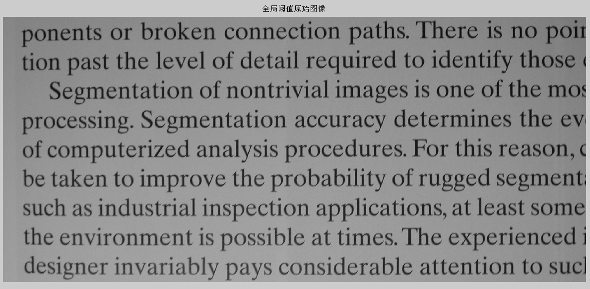
[H,theta,rho]=hough(f);figure,imshow(theta,rho,H,[],'notruesize');%为什么显示不出来呢axis on,axis normal;xlabel('\theta'),ylabel('\rho');%% 计算全局阈值clcclearf = imread('.\images\dipum_images_ch10\Fig1013(a)(scanned-text-grayscale).tif');imshow(f);title('全局阈值原始图像')162%其图片显示结果如下：

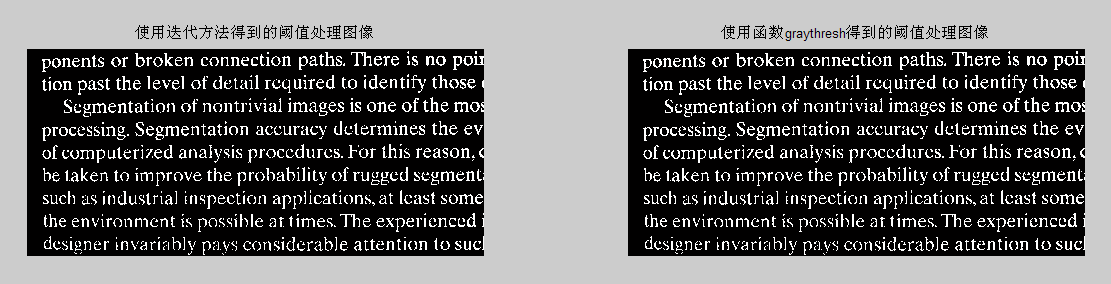
T=0.5*(double(min(f(:)))+double(max(f(:))));done=false;while ~done g=f>=T; Tnext=0.5*(mean(f(g))+mean(f(~g))); done=abs(T-Tnext)<0.5 T=Tnext;endg=f<=T;%因为前景是黑色的字，所以要分离出来的话这里就要用<=.figure,subplot(121),imshow(g);title('使用迭代方法得到的阈值处理图像');T2=graythresh(f);%得到的是0~1的小数？g=f<=T2*255;subplot(122),imshow(g);title('使用函数graythresh得到的阈值处理图像');181%阈值处理后结果如下：

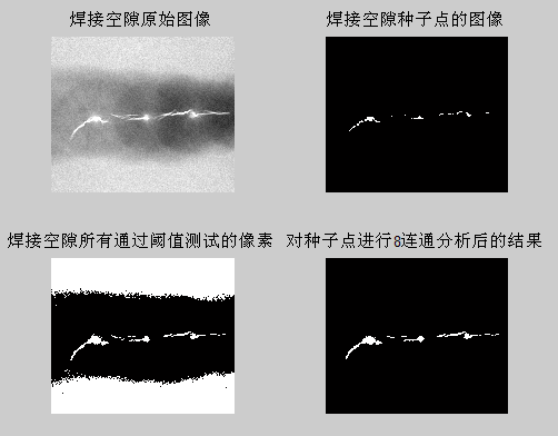
%% 焊接空隙区域生长clcclearf = imread('.\images\dipum_images_ch10\Fig1014(a)(defective_weld).tif');subplot(221),imshow(f);title('焊接空隙原始图像');%函数regiongrow返回的NR为是不同区域的数目，参数SI是一副含有种子点的图像%TI是包含在经过连通前通过阈值测试的像素[g,NR,SI,TI]=regiongrow(f,255,65);%种子的像素值为255，65为阈值subplot(222),imshow(SI);title('焊接空隙种子点的图像');subplot(223),imshow(TI);title('焊接空隙所有通过阈值测试的像素');subplot(224),imshow(g);title('对种子点进行8连通分析后的结果');202%焊接空隙区域生长图如下：

%% 使用区域分离和合并的图像分割clcclearf = imread('.\images\dipum_images_ch10\Fig1017(a)(cygnusloop_Xray_original).tif');subplot(231),imshow(f);title('区域分割原始图像');g32=splitmerge(f,32,@predicate);%32代表分割中允许最小的块subplot(232),imshow(g32);title('mindim为32时的分割图像');g16=splitmerge(f,16,@predicate);%32代表分割中允许最小的块subplot(233),imshow(g16);title('mindim为32时的分割图像');g8=splitmerge(f,8,@predicate);%32代表分割中允许最小的块subplot(234),imshow(g8);title('mindim为32时的分割图像');g4=splitmerge(f,4,@predicate);%32代表分割中允许最小的块subplot(235),imshow(g4);title('mindim为32时的分割图像');g2=splitmerge(f,2,@predict);%32代表分割中允许最小的块subplot(236),imshow(g2);title('mindim为32时的分割图像');%% 使用距离和分水岭变换分割灰度图像clcclearf = imread('.\images\dipum_images_ch10\Fig0925(a)(dowels).tif');subplot(231),imshow(f);title('使用距离和分水岭分割原图');g=im2bw(f,graythresh(f));subplot(232),imshow(g),title('原图像阈值处理后的图像');gc=~g;subplot(233),imshow(gc),title('阈值处理后取反图像');D=bwdist(gc);subplot(234),imshow(D),title('使用距离变换后的图像');L=watershed(-D);w=L==0;subplot(235),imshow(w),title('距离变换后的负分水岭图像');g2=g & ~w;subplot(236),imshow(g2),title('阈值图像与分水岭图像相与图像');252%使用距离分水岭图像如下：

%% 使用梯度和分水岭变换分割灰度图像clcclearf = imread('.\images\dipum_images_ch10\Fig1021(a)(small-blobs).tif');subplot(221),imshow(f);title('使用梯度和分水岭变换分割灰度图像');h=fspecial('sobel');fd=double(f);g=sqrt(imfilter(fd,h,'replicate').^2+imfilter(fd,h','replicate').^2);subplot(222),imshow(g,[]);title('使用梯度和分水岭分割幅度图像');L=watershed(g);wr=L==0;subplot(223),imshow(wr);title('对梯度复制图像进行二值分水岭后图像');g2=imclose(imopen(g,ones(3,3)),ones(3,3));L2=watershed(g2);wr2=L2==0;f2=f;f2(wr2)=255;subplot(224),imshow(f2);title('平滑梯度图像后的分水岭变换');279%使用梯度和分水岭变换分割灰度图像结果如下：

%% 控制标记符的分水岭分割clcclearf = imread('.\images\dipum_images_ch10\Fig1022(a)(gel-image).tif');imshow(f);title('控制标记符的分水岭分割原图像');h=fspecial('sobel');fd=double(f);g=sqrt(imfilter(fd,h,'replicate').^2+imfilter(fd,h','replicate').^2);L=watershed(g);wr=L==0;figure,subplot(231),imshow(wr,[]);title('控制标记符的分水岭分割幅度图像');

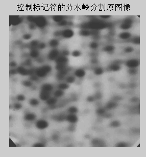
rm=imregionalmin(g);%梯度图像有很多较浅的坑，造成的原因是原图像不均匀背景中灰度细小的变化subplot(232),imshow(rm,[]);title('对梯度幅度图像的局部最小区域');im=imextendedmin(f,2);%得到内部标记符fim=f;fim(im)=175;subplot(233),imshow(f,[]);title('内部标记符');Lim=watershed(bwdist(im));em=Lim==0;subplot(234),imshow(em,[]);title('外部标记符');g2=imimposemin(g,im | em);subplot(235),imshow(g2,[]);title('修改后的梯度幅度值');L2=watershed(g2);f2=f;f2(L2==0)=255;subplot(236),imshow(f2),title('最后分割的结果');319%控制标记符的分水岭分割过程如下：

<img src="https://img-blog.csdn.net/20141215152203984" alt="" />

<span style="color: rgb(75, 75, 75); font-family: Verdana, Geneva, Arial, Helvetica, sans-serif; font-size: 13px; line-height: 19.5px;">作者：tornadomeet 出处：</span><a target=_blank class="smarterwiki-linkify" href="http://www.cnblogs.com/tornadomeet" style="color: rgb(26, 139, 200); text-decoration: none; font-family: Verdana, Geneva, Arial, Helvetica, sans-serif; font-size: 13px; line-height: 19.5px;">http://www.cnblogs.com/tornadomeet</a><span style="color: rgb(75, 75, 75); font-family: Verdana, Geneva, Arial, Helvetica, sans-serif; font-size: 13px; line-height: 19.5px;"> </span>