混沌系统数值模拟

4阶 龙格库塔方法

import numpy as np
import matplotlib.pyplot as plt
%matplotlib inline
from mpl_toolkits.mplot3d import Axes3D
from math import *

def dxdt(x,y,z,h=2e-2):

    K1, L1, M1 = f1(x,y,z), f2(x,y,z), f3(x,y,z)
    dx, dy, dz = h*K1/2, h*L1/2, h*M1/2
    K2, L2, M2 = f1(x+dx,y+dy, z+dz), f2(x+dx,y+dy, z+dz), f3(x+dx,y+dy, z+dz) 
    dx, dy, dz = h*K2/2, h*L2/2, h*M2/2
    K3, L3, M3 = f1(x+dx,y+dy, z+dz), f2(x+dx,y+dy, z+dz), f3(x+dx,y+dy, z+dz)
    dx, dy, dz = h*K3, h*L3, h*M3  
    K4, L4, M4 = f1(x+dx,y+dy, z+dz), f2(x+dx,y+dy, z+dz), f3(x+dx,y+dy, z+dz)

    dx = (K1 + 2*K2 + 2*K3 + K4)*h/6
    dy = (L1 + 2*L2 + 2*L3 + L4)*h/6
    dz = (M1 + 2*M2 + 2*M3 + M4)*h/6
    return dx, dy, dz

def trajectory(initial_point = [0.1, 0.1, 0.1], num_points=1e4, h=2e-2):
    x0, y0, z0 = initial_point[0], initial_point[1], initial_point[2]
    n = int(num_points)
    x = np.zeros([n,3])
    x[0,:] = [x0,y0,z0]

    for k in range(1,n):
        dx,dy,dz = dxdt(x[k-1,0],x[k-1,1],x[k-1,2],h)
        x[k,0] = x[k-1,0] + dx
        x[k,1] = x[k-1,1] + dy
        x[k,2] = x[k-1,2] + dz

    return x.T

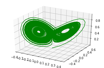
洛伦兹系统

def f1(x,y,z):
    A = 10
    return A*(y - x)


def f2(x,y,z):
    B = 28;
    return B*x - y - x*z;
    

def f3(x,y,z):
    C = 8/3
    return x*y - C*z


N = 5000
scale  = 50
x = trajectory([0.1,0.100001,0.1],N)/scale
x_ = trajectory([0.1, 0.1, 0.1],num_points=N)/scale
fig = plt.figure()
ax = fig.add_subplot(111, projection='3d')
plt.plot(*x, 'g')
plt.show()
plt.subplot(3,1,1)
plt.plot(x[0], 'r'), plt.plot(x_[0], 'g')
plt.subplot(3,1,2)
plt.plot(x[1], 'r'), plt.plot(x_[1], 'g')
plt.subplot(3,1,3)
plt.plot(x[2], 'r'), plt.plot(x_[2], 'g')
plt.show()

Rossler 系统

def f1(x,y,z):
    return -y-z

def f2(x,y,z):
    A = 0.25
    return x + A*y
    
def f3(x,y,z):
    B = 1
    C = 5
    return B + z*(x - C)

N = 10000
scale  = 5
x = trajectory([0.10001,0.1,0.1],N)/scale
x_ = trajectory([0.1, 0.1, 0.1],num_points=N)/scale
fig = plt.figure()
ax = fig.add_subplot(111, projection='3d')
plt.plot(*x, 'g')
plt.show()
plt.subplot(3,1,1)
plt.plot(x[0], 'r'), plt.plot(x_[0], 'g')
plt.subplot(3,1,2)
plt.plot(x[1], 'r'), plt.plot(x_[1], 'g')
plt.subplot(3,1,3)
plt.plot(x[2], 'r'), plt.plot(x_[2], 'g')
plt.show()

Chua 系统

def g(x):
    return 0.6*x -1.1*x*fabs(x) + 0.45*x**3

a = 12.8
b = 19.1
x0, y0, z0 = 1.7, 0.0, -1.9

def f1(x,y,z):
    return a*(y -g(x))

def f2(x,y,z):
    return x - y + z
    
def f3(x,y,z):
    return -b*y


N = 10000
scale  = 5
x = trajectory([0.1,0.1,0.1],N)/scale
x_ = trajectory([1, 1, 1],num_points=N)/scale
fig = plt.figure()
ax = fig.add_subplot(111, projection='3d')
plt.plot(*x_, 'g')
plt.plot(*x, 'r')
plt.show()
plt.subplot(3,1,1)
plt.plot(x[0], 'r')
# plt.plot(x_[0], 'g')
plt.subplot(3,1,2)
plt.plot(x[1], 'r')
# plt.plot(x_[1], 'g')
plt.subplot(3,1,3)
plt.plot(x[2], 'r')
# plt.plot(x_[2], 'g')
plt.show()

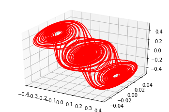
Chen 系统

a=40.
b=3.
c=28.
step=0.002
x0=-0.1
y0=0.5
z0=-0.6


def f1(x,y,z):
    return a*(y - x)

def f2(x,y,z):
    return (c-a)*x - x*z + c*y
    
def f3(x,y,z):
    return x*y - b*z

N = 10000
scale  = 5
x = trajectory([x0, y0, z0],N,step)/scale
x_ = trajectory([x0+0.001, y0, z0],N,step)/scale
fig = plt.figure()
ax = fig.add_subplot(111, projection='3d')
plt.plot(*x, 'r')
plt.show()
plt.subplot(3,1,1)
plt.plot(x[0], 'r'), plt.plot(x_[0], 'g')
plt.subplot(3,1,2)
plt.plot(x[1], 'r'), plt.plot(x_[1], 'g')
plt.subplot(3,1,3)
plt.plot(x[2], 'r'), plt.plot(x_[2], 'g')
plt.show()

Rabinovich-Fabrikant 系统

ParamA = 1.1
ParamB = 0.87

def f1(x,y,z):
    return y*(z - 1 + x*x) + ParamB*x

def f2(x,y,z):
    return x*(3*z + 1 - x*x) + ParamB*y
    
def f3(x,y,z):
    return -2*z*(ParamA + x*y)

N = 5000
scale  = 5
x = trajectory([-1,0,0.5],N,h=2e-2)/scale
x_ = trajectory([-1,0.001,0.5],N,h=2e-2)/scale
fig = plt.figure()
ax = fig.add_subplot(111, projection='3d')
plt.plot(*x, 'r')
plt.show()
plt.subplot(3,1,1)
plt.plot(x[0], 'r'), plt.plot(x_[0], 'g')
plt.subplot(3,1,2)
plt.plot(x[1], 'r'), plt.plot(x_[1], 'g')
plt.subplot(3,1,3)
plt.plot(x[2], 'r'), plt.plot(x_[2], 'g')
plt.show()