竞赛 基于LSTM的天气预测 - 时间序列预测

0 前言

🔥 优质竞赛项目系列，今天要分享的是

机器学习大数据分析项目

该项目较为新颖，适合作为竞赛课题方向，学长非常推荐！

🧿 更多资料, 项目分享：

https://gitee.com/dancheng-senior/postgraduate

---

1 数据集介绍

​
df = pd.read_csv(‘/home/kesci/input/jena1246/jena_climate_2009_2016.csv’)
df.head()

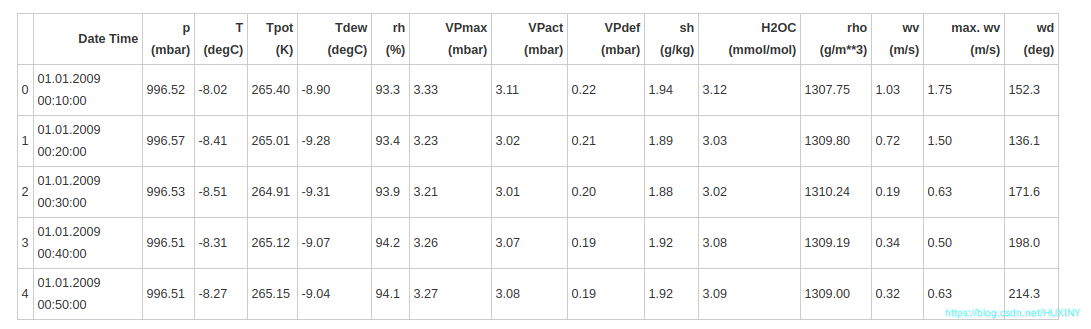
如上所示，每10分钟记录一次观测值，一个小时内有6个观测值，一天有144（6x24）个观测值。

给定一个特定的时间，假设要预测未来6小时的温度。为了做出此预测，选择使用5天的观察时间。因此，创建一个包含最后720（5x144）个观测值的窗口以训练模型。

下面的函数返回上述时间窗以供模型训练。参数 history_size 是过去信息的滑动窗口大小。target_size
是模型需要学习预测的未来时间步，也作为需要被预测的标签。

下面使用数据的前300,000行当做训练数据集，其余的作为验证数据集。总计约2100天的训练数据。

​
def univariate_data(dataset, start_index, end_index, history_size, target_size):
data = []
labels = []

    start_index = start_index + history_size
    if end_index is None:
        end_index = len(dataset) - target_size

    for i in range(start_index, end_index):
        indices = range(i-history_size, i)
        # Reshape data from (history`1_size,) to (history_size, 1)
        data.append(np.reshape(dataset[indices], (history_size, 1)))
        labels.append(dataset[i+target_size])
    return np.array(data), np.array(labels)

2 开始分析

2.1 单变量分析

首先，使用一个特征（温度）训练模型，并在使用该模型做预测。

2.1.1 温度变量

从数据集中提取温度

​
uni_data = df[‘T (degC)’]
uni_data.index = df[‘Date Time’]
uni_data.head()

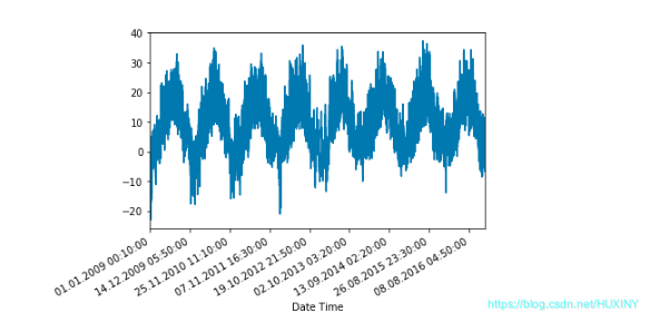
观察数据随时间变化的情况

进行标准化

​
#标准化
uni_train_mean = uni_data[:TRAIN_SPLIT].mean()
uni_train_std = uni_data[:TRAIN_SPLIT].std()

uni_data = (uni_data-uni_train_mean)/uni_train_std
#写函数来划分特征和标签
univariate_past_history = 20
univariate_future_target = 0
x_train_uni, y_train_uni = univariate_data(uni_data, 0, TRAIN_SPLIT, # 起止区间
                                           univariate_past_history,
                                           univariate_future_target)
x_val_uni, y_val_uni = univariate_data(uni_data, TRAIN_SPLIT, None,
                                       univariate_past_history,
                                       univariate_future_target)

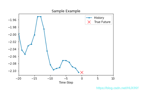
可见第一个样本的特征为前20个时间点的温度，其标签为第21个时间点的温度。根据同样的规律，第二个样本的特征为第2个时间点的温度值到第21个时间点的温度值，其标签为第22个时间点的温度……

2.2 将特征和标签切片

​
BATCH_SIZE = 256
BUFFER_SIZE = 10000

train_univariate = tf.data.Dataset.from_tensor_slices((x_train_uni, y_train_uni))
train_univariate = train_univariate.cache().shuffle(BUFFER_SIZE).batch(BATCH_SIZE).repeat()

val_univariate = tf.data.Dataset.from_tensor_slices((x_val_uni, y_val_uni))
val_univariate = val_univariate.batch(BATCH_SIZE).repeat()

2.3 建模

​
simple_lstm_model = tf.keras.models.Sequential([
tf.keras.layers.LSTM(8, input_shape=x_train_uni.shape[-2:]), # input_shape=(20,1) 不包含批处理维度
tf.keras.layers.Dense(1)
])

simple_lstm_model.compile(optimizer='adam', loss='mae')

2.4 训练模型

​
EVALUATION_INTERVAL = 200
EPOCHS = 10

simple_lstm_model.fit(train_univariate, epochs=EPOCHS,
                      steps_per_epoch=EVALUATION_INTERVAL,
                      validation_data=val_univariate, validation_steps=50)

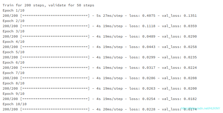
训练过程

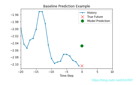
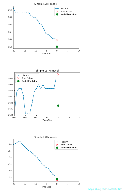
训练结果 - 温度预测结果

2.5 多变量分析

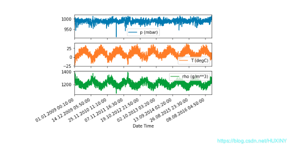
在这里，我们用过去的一些压强信息、温度信息以及密度信息来预测未来的一个时间点的温度。也就是说，数据集中应该包括压强信息、温度信息以及密度信息。

2.5.1 压强、温度、密度随时间变化绘图

2.5.2 将数据集转换为数组类型并标准化

​
dataset = features.values
data_mean = dataset[:TRAIN_SPLIT].mean(axis=0)
data_std = dataset[:TRAIN_SPLIT].std(axis=0)

dataset = (dataset-data_mean)/data_std

def multivariate_data(dataset, target, start_index, end_index, history_size,
                      target_size, step, single_step=False):
    data = []
    labels = []

    start_index = start_index + history_size
    
    if end_index is None:
        end_index = len(dataset) - target_size

    for i in range(start_index, end_index):
        indices = range(i-history_size, i, step) # step表示滑动步长
        data.append(dataset[indices])

        if single_step:
            labels.append(target[i+target_size])
        else:
            labels.append(target[i:i+target_size])

    return np.array(data), np.array(labels)

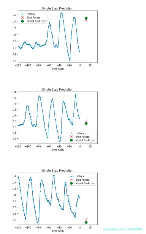
2.5.3 多变量建模训练训练

​

    single_step_model = tf.keras.models.Sequential()
    single_step_model.add(tf.keras.layers.LSTM(32,
                                               input_shape=x_train_single.shape[-2:]))
    single_step_model.add(tf.keras.layers.Dense(1))
    
    single_step_model.compile(optimizer=tf.keras.optimizers.RMSprop(), loss='mae')
    
    single_step_history = single_step_model.fit(train_data_single, epochs=EPOCHS,
                                                steps_per_epoch=EVALUATION_INTERVAL,
                                                validation_data=val_data_single,
                                                validation_steps=50)


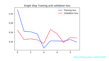
    def plot_train_history(history, title):
        loss = history.history['loss']
        val_loss = history.history['val_loss']
    
        epochs = range(len(loss))
    
        plt.figure()
    
        plt.plot(epochs, loss, 'b', label='Training loss')
        plt.plot(epochs, val_loss, 'r', label='Validation loss')
        plt.title(title)
        plt.legend()
    
        plt.show()

    plot_train_history(single_step_history,
                       'Single Step Training and validation loss')

6 最后

🧿 更多资料, 项目分享：

https://gitee.com/dancheng-senior/postgraduate