R programming - swirl learning

open swirl

> library(swirl)
> swirl()

1. The basics of programming in R

If at any point you’d like more information on a particular topic related to R, you can type help.start() at the prompt, which will open a menu of resources (either within RStudio or your default web browser, depending on your setup).

> 5 + 7
[1] 12
> x <- 5+7
> x
[1] 12
> y <- x-3
> > y
[1] 9
> z <- c(1.1, 9, 3.14)  ## create a vector is with the c() function, which stands for 'concatenate' or 'combine'.
> ?c ## have questions about a particular function, you can access R's built-in help files via the `?` command
> z
[1] 1.10 9.00 3.14
> c(z, 555)
[1]   1.10   9.00   3.14 555.00
> c(z, 555, z)
[1]   1.10   9.00   3.14 555.00   1.10   9.00   3.14
> z * 2 +100
[1] 102.20 118.00 106.28
> my_sqrt <- sqrt(z-1)  ## take the square root, use the sqrt(), take the absolute value, use the abs() function
> my_sqrt
[1] 0.3162278 2.8284271 1.4628739
> my_div <- z / my_sqrt
> my_div
[1] 3.478505 3.181981 2.146460  ## When given two vectors of the same length, R simply performs the specified arithmetic operation (`+`, `-`, `*`, etc.)element-by-element. If the vectors are of different lengths, R 'recycles' the shorter vector until it is the same length as the longer vector.
> c(1, 2, 3, 4) + c(0, 10)
[1]  1 12  3 14
> c(1, 2, 3, 4) + c(0, 10, 100)
[1]   1  12 103   4
> z * 2 +100
[1] 102.20 118.00 106.28
> z * 2 +1000
[1] 1002.20 1018.00 1006.28
> my_div
[1] 3.478505 3.181981 2.146460

2. Workspace and Files

> getwd()   ## Determine which directory your R session is using as its current working directory using getwd()
[1] "/home/rstudio"
> ls()     ## List all the objects in your local workspace using ls()
[1] "my_div"  "my_sqrt" "x"       "y"       "z"
> list.files()  ## List all the files in your working directory using list.files() or dir()
[1] "Getting Started with Your Lab.rd" "R_Programming.swc"                "README.rd"                       
[4] "Week 1"                           "Week 2"                           "Week 3"                          
[7] "Week 4" 
> args(list.files)  ## Use the args() function to determine the arguments to list.files()
function (path = ".", pattern = NULL, all.files = FALSE, full.names = FALSE, 
    recursive = FALSE, ignore.case = FALSE, include.dirs = FALSE, 
    no.. = FALSE) 
NULL
> old.dir <- getwd() ## assign the value of the current working directory to a variable called "old.dir"
> dir.create("testdir")  ## create a directory in the current working directory called "testdir"
> setwd("testdir")   ## Set your working directory to "testdir" with the setwd() command
> file.create("mytest.R")  ## Create a file in your working directory called "mytest.R" using the file.create() function
[1] TRUE
> list.files()  ## listing all the files in the current directory
[1] "mytest.R"
> file.exists("mytest.R")  ## Check to see if "mytest.R" exists in the working directory using the file.exists() function
[1] TRUE
> file.info("mytest.R")  ## Access information about the file "mytest.R" by using file.info()
         size isdir mode               mtime               ctime               atime  uid  gid   uname  grname
mytest.R    0 FALSE  644 2022-05-10 11:47:14 2022-05-10 11:47:14 2022-05-10 11:47:14 1000 1000 rstudio rstudio

## use the $ operator --- e.g., file.info("mytest.R")$mode --- to grab specific items
> file.rename("mytest.R", "mytest2.R") ## Change the name of the file "mytest.R" to "mytest2.R"
[1] TRUE
> file.copy("mytest2.R", "mytest3.R") ## Make a copy of "mytest2.R" called "mytest3.R"
[1] TRUE
> file.path("mytest3.R")  ## Provide the relative path to the file "mytest3.R"
[1] "mytest3.R"

## construct file and directory paths that are independent of the operating system your R code is running on
> file.path("folder1", "folder2")  ## Pass 'folder1' and 'folder2' as arguments to file.path to make a platform-independent pathname
[1] "folder1/folder2"
> dir.create(file.path("testdir2", "testdir3"), recursive = TRUE) ## Create a directory in the current working directory called "testdir2" and a subdirectory for it called "testdir3"
> setwd(old.dir) ## save the settings that you had before you began an analysis and then go back to them at the end

3. Sequences of Numbers

> 1:20   # create a sequence of numbers in R is by using the `:` operator
 [1]  1  2  3  4  5  6  7  8  9 10 11 12 13 14 15 16 17 18 19 20
> pi:10  # create a sequence of real numbers
[1] 3.141593 4.141593 5.141593 6.141593 7.141593 8.141593 9.141593
> ?`:` # have questions about a particular R function, you can access its documentation with a question mark followed by the function name: ?function_name_here
> seq(1,20) # seq() does exactly the same thing as the `:` operator
 [1]  1  2  3  4  5  6  7  8  9 10 11 12 13 14 15 16 17 18 19 20
> my_seq <- seq(5,10,length=30) # a sequence of 30 numbers between 5 and 10
> length(my_seq) # confirm that my_seq has length 30 
[1] 30
> 1:length(my_seq) # combine the `:` operator and the length() function
 [1]  1  2  3  4  5  6  7  8  9 10 11 12 13 14 15 16 17 18 19 20 21 22 23 24 25 26 27 28 29 30
 > seq(along.with=my_seq)
 [1]  1  2  3  4  5  6  7  8  9 10 11 12 13 14 15 16 17 18 19 20 21 22 23 24 25 26 27 28 29 30
 > seq_along(my_seq)
 [1]  1  2  3  4  5  6  7  8  9 10 11 12 13 14 15 16 17 18 19 20 21 22 23 24 25 26 27 28 29 30
 > rep(0, times=40) # creating a vector that contains 40 zeros
 [1] 0 0 0 0 0 0 0 0 0 0 0 0 0 0 0 0 0 0 0 0 0 0 0 0 0 0 0 0 0 0 0 0 0 0 0 0 0 0 0 0
 > rep(c(0,1,2), times=10) #contain 10 repetitions of the vector (0, 1, 2)
 [1] 0 1 2 0 1 2 0 1 2 0 1 2 0 1 2 0 1 2 0 1 2 0 1 2 0 1 2 0 1 2
 > rep(c(0,1,2), each=10) # vector to contain 10 zeros, then 10 ones, then 10 twos
 [1] 0 0 0 0 0 0 0 0 0 0 1 1 1 1 1 1 1 1 1 1 2 2 2 2 2 2 2 2 2 2

4. Vectors

>  c(0.5,55,-10,6)
[1]   0.5  55.0 -10.0   6.0
> num_vect <- c(0.5,55,-10,6)
> tf <- num_vect < 1
> tf
[1]  TRUE FALSE  TRUE FALSE
> num_vect >= 6
[1] FALSE  TRUE FALSE  TRUE
## The `<` and `>=` symbols in these examples are called 'logical operators'. Other logical operators include `>`, `<=`, `==` for exact equality, and `!=` for inequality.

## If we have two logical expressions, A and B, we can ask whether at least one is TRUE with A | B (logical 'or' a.k.a. 'union') or whether they are both TRUE with A & B (logical 'and' a.k.a. 'intersection'). Lastly, !A is the negation of A and is TRUE when A is FALSE and vice versa.

> my_char <- c("My", "name", "is")
> my_char
[1] "My"   "name" "is" 
> paste(my_char, collapse = " ") ## join the elements of my_char together into one continuous character string
[1] "My name is"
> my_name <- c(my_char, "your_name_here")
> my_name
[1] "My"             "name"           "is"             "your_name_here"
> paste(my_name, collapse=" ")
[1] "My name is your_name_here"
> paste("Hello", "world!", sep=" ")
[1] "Hello world!"
> paste(1:3, c("X","Y","Z"), sep="") ## join two vectors
[1] "1X" "2Y" "3Z"
> paste(LETTERS, 1:4, sep="-")  ## Since the character vector LETTERS is longer than the numeric vector 1:4, R simply recycles, or repeats, 1:4 until it matches the length of LETTERS.
 [1] "A-1" "B-2" "C-3" "D-4" "E-1" "F-2" "G-3" "H-4" "I-1" "J-2" "K-3"
[12] "L-4" "M-1" "N-2" "O-3" "P-4" "Q-1" "R-2" "S-3" "T-4" "U-1" "V-2"
[23] "W-3" "X-4" "Y-1" "Z-2"

5. Missing Values

> x <- c(44, NA, 5, NA)
> x * 3
[1] 132  NA  15  NA
> y <- rnorm(1000) ## create a vector containing 1000 draws from a standard normal distribution
> z <- rep(NA, 1000) ## create a vector containing 1000 NAs
> my_data <- sample(c(y, z), 100) ## select 100 elements at random from these 2000 values (combining y and z) such that we don't know how many NAs
> my_na <- is.na(my_data) ## whether each element of a vector is NA
> my_na
  [1] FALSE FALSE  TRUE FALSE FALSE FALSE FALSE  TRUE  TRUE FALSE  TRUE
 [12] FALSE  TRUE FALSE FALSE  TRUE FALSE FALSE  TRUE  TRUE FALSE FALSE
 [23]  TRUE FALSE FALSE FALSE  TRUE FALSE FALSE  TRUE FALSE  TRUE  TRUE
 [34]  TRUE  TRUE FALSE  TRUE  TRUE  TRUE FALSE FALSE  TRUE FALSE FALSE
 [45] FALSE FALSE FALSE FALSE FALSE  TRUE FALSE  TRUE FALSE FALSE  TRUE
 [56] FALSE  TRUE  TRUE FALSE  TRUE  TRUE  TRUE FALSE FALSE FALSE  TRUE
 [67]  TRUE  TRUE  TRUE FALSE  TRUE  TRUE FALSE FALSE FALSE  TRUE  TRUE
 [78]  TRUE  TRUE FALSE FALSE  TRUE FALSE FALSE  TRUE FALSE  TRUE FALSE
 [89] FALSE  TRUE  TRUE  TRUE FALSE  TRUE  TRUE  TRUE  TRUE  TRUE  TRUE
[100]  TRUE
> sum(my_na) ## R represents TRUE as the number 1 and FALSE as the number 0, count the total number of TRUEs in my_na
[1] 50
> my_data
  [1]  0.12455323  0.67423423          NA -0.48260297  0.97958115
  [6] -1.20435478 -0.01913248          NA          NA  0.10018291
 [11]          NA -1.08463248          NA  2.13408186  0.18073727
 [16]          NA -0.01183309 -0.32764262          NA          NA
 [21]  2.63247946  0.01587571          NA -0.41318789 -0.29861956
 [26] -0.44485629          NA -1.18701096  0.64935527          NA
 [31] -1.49390267          NA          NA          NA          NA
 [36] -1.50756965          NA          NA          NA -0.09745191
 [41] -0.07975442          NA -0.41299064  0.34577227 -0.46547004
 [46]  0.04980392  1.77753482  0.90347037 -0.10886004          NA
 [51] -0.58566588          NA  1.12031568 -0.21611369          NA
 [56] -0.54257504          NA          NA -0.43416869          NA
 [61]          NA          NA  1.03016896 -0.42783936  1.12238303
 [66]          NA          NA          NA          NA -0.96768938
 [71]          NA          NA -1.48739369  0.53381752 -0.10638435
 [76]          NA          NA          NA          NA  0.80668825
 [81] -2.06580872          NA -1.27188173  0.43625778          NA
 [86] -1.25152733          NA  1.82897996  1.59659763          NA
 [91]          NA          NA -1.39135059          NA          NA
 [96]          NA          NA          NA          NA          NA
> 0 / 0
[1] NaN
> Inf - Inf
[1] NaN

6. Subsetting Vectors

> x
 [1]         NA         NA         NA  0.4010469 -0.3557759         NA
 [7]         NA -1.1525077         NA -0.2966289         NA         NA
[13] -0.1374056 -0.8698718         NA -0.8308277         NA         NA
[19] -0.1461715 -1.4897203  1.2523480         NA  1.2570167         NA
[25] -0.1316774         NA  0.3537307 -0.2806951         NA         NA
[31]  0.2424451 -0.4498029         NA         NA         NA -1.2609592
[37]         NA  3.3100256  0.5122851 -0.9446367
> x[1:10] ## view the first ten elements of x
 [1]         NA         NA         NA  0.4010469 -0.3557759         NA
 [7]         NA -1.1525077         NA -0.2966289
> x[is.na(x)] ##  A vector of all NAs
 [1] NA NA NA NA NA NA NA NA NA NA NA NA NA NA NA NA NA NA NA NA
> y <- x[!is.na(x)] ## contains all of the non-NA values from x
> y
 [1]  0.4010469 -0.3557759 -1.1525077 -0.2966289 -0.1374056 -0.8698718
 [7] -0.8308277 -0.1461715 -1.4897203  1.2523480  1.2570167 -0.1316774
[13]  0.3537307 -0.2806951  0.2424451 -0.4498029 -1.2609592  3.3100256
[19]  0.5122851 -0.9446367
> y[y>0] ## the positive elements of our original vector x
[1] 0.4010469 1.2523480 1.2570167 0.3537307 0.2424451 3.3100256 0.5122851
> x[x>0] ## isolate the positive elements of x
 [1]        NA        NA        NA 0.4010469        NA        NA
 [7]        NA        NA        NA        NA        NA        NA
[13] 1.2523480        NA 1.2570167        NA        NA 0.3537307
[19]        NA        NA 0.2424451        NA        NA        NA
[25]        NA 3.3100256 0.5122851
> x[!is.na(x) & x>0]
[1] 0.4010469 1.2523480 1.2570167 0.3537307 0.2424451 3.3100256 0.5122851

## R uses 'one-based indexing', which (you guessed it!) means the first element of a vector is considered element 1. subset the 3rd, 5th, and 7th elements of x
> x[c(3,5,7)]
[1]         NA -0.3557759         NA
> x[0]
numeric(0)
> x[3000]
[1] NA

## Whereas x[c(2, 10)] gives us ONLY the 2nd and 10th elements of x, x[c(-2, -10)] gives us all elements of x EXCEPT for the 2nd and 10 elements
> x[c(-2,-10)]
 [1]         NA         NA  0.4010469 -0.3557759         NA         NA
 [7] -1.1525077         NA         NA         NA -0.1374056 -0.8698718
[13]         NA -0.8308277         NA         NA -0.1461715 -1.4897203
[19]  1.2523480         NA  1.2570167         NA -0.1316774         NA
[25]  0.3537307 -0.2806951         NA         NA  0.2424451 -0.4498029
[31]         NA         NA         NA -1.2609592         NA  3.3100256
[37]  0.5122851 -0.9446367

> x[-c(2,10)] ## A shorthand way of specifying multiple negative numbers is to put the negative sign out in front of the vector of positive numbers
 [1]         NA         NA  0.4010469 -0.3557759         NA         NA
 [7] -1.1525077         NA         NA         NA -0.1374056 -0.8698718
[13]         NA -0.8308277         NA         NA -0.1461715 -1.4897203
[19]  1.2523480         NA  1.2570167         NA -0.1316774         NA
[25]  0.3537307 -0.2806951         NA         NA  0.2424451 -0.4498029
[31]         NA         NA         NA -1.2609592         NA  3.3100256
[37]  0.5122851 -0.9446367
> vect <- c(foo=11, bar=2, norf=NA)
> vect
 foo  bar norf 
  11    2   NA
> names(vect) ## get the names of vect by passing vect as an argument to the names() function
[1] "foo"  "bar"  "norf"
> vect2 <- c(11, 2, NA)
> names(vect2) <- c("foo", "bar", "norf")
> identical(vect, vect2)
[1] TRUE

7. Matrices and Data Frames

> my_vector <- 1:20 ## create a vector containing the numbers 1 through 20
> my_vector
 [1]  1  2  3  4  5  6  7  8  9 10 11 12 13 14 15 16 17 18 19 20
 ## The dim() function tells us the 'dimensions' of an object 
> dim(my_vector) ## my_vector is a vector, it doesn't have a `dim` attribute (so it's just NULL)
NULL
> length(my_vector) ## find its length using the length() function
[1] 20
> dim(my_vector) <- c(4,5) ## dim() function allows you to get OR set the `dim` attribute for an R object
> dim(my_vector) ## Use dim(my_vector) to confirm that we've set the `dim` attribute correctly
[1] 4 5
> attributes(my_vector) ## Another way to see this is by calling the attributes() function
$dim
[1] 4 5
> my_vector
     [,1] [,2] [,3] [,4] [,5]
[1,]    1    5    9   13   17
[2,]    2    6   10   14   18
[3,]    3    7   11   15   19
[4,]    4    8   12   16   20
> class(my_vector)
[1] "matrix" "array" 
> my_matrix <- my_vector
> my_matrix2 <- matrix(1:20, 4, 5)
> identical(my_matrix, my_matrix2)
[1] TRUE
> patients <- c("Bill", "Gina", "Kelly", "Sean") ## creating a character vector containing the names of our patients -- Bill, Gina, Kelly, and Sean
> cbind(patients, my_matrix)
     patients                       
[1,] "Bill"   "1" "5" "9"  "13" "17"
[2,] "Gina"   "2" "6" "10" "14" "18"
[3,] "Kelly"  "3" "7" "11" "15" "19"
[4,] "Sean"   "4" "8" "12" "16" "20"

##  It appears that combining the character vector with our matrix of numbers caused everything to be enclosed in double quotes. This means we're left with a matrix of character strings, which is no good.

## matrices can only contain ONE class of data. Therefore, when we tried to combine a character vector with a numeric matrix, R was forced to 'coerce' the numbers to characters, hence the double quotes.
> my_data <- data.frame(patients, my_matrix)
> my_data
  patients X1 X2 X3 X4 X5
1     Bill  1  5  9 13 17
2     Gina  2  6 10 14 18
3    Kelly  3  7 11 15 19
4     Sean  4  8 12 16 20
> class(my_data)
[1] "data.frame"
> cnames <- c("patient", "age", "weight", "bp", "rating", "test") ## create a vector containing one element for each column. Create a character vector called cnames that contains the following values (in order) -- "patient", "age", "weight", "bp", "rating", "test".
> colnames(my_data) <- cnames ## use the colnames() function to set the `colnames` attribute for our data frame
> my_data
  patient age weight bp rating test
1    Bill   1      5  9     13   17
2    Gina   2      6 10     14   18
3   Kelly   3      7 11     15   19
4    Sean   4      8 12     16   20

8. Logic

> TRUE == TRUE
[1] TRUE
> FALSE == FALSE
[1] TRUE
> (FALSE == TRUE) == FALSE
[1] TRUE
> 6 == 7
[1] FALSE
> 6 <= 7
[1] TRUE
> 6 <7 
[1] TRUE
> 10 <= 10
[1] TRUE
> 5 != 7 ## 'not equals' operator represented by `!=`
[1] TRUE
> FALSE & FALSE
[1] FALSE
> TRUE & c(TRUE, FALSE, FALSE) ## the `&` operator to evaluate AND across a vector
[1]  TRUE FALSE FALSE
> TRUE && c(TRUE, FALSE, FALSE) ## The `&&` version of AND only evaluates the first member of a vector
[1] TRUE
> TRUE | c(TRUE, FALSE, FALSE) ## `|` version of OR evaluates OR across an entire vector
[1] TRUE TRUE TRUE
> TRUE || c(TRUE, FALSE, FALSE) ## the `||` version of OR only evaluates the first member of a vector
## An expression using the OR operator will evaluate to TRUE if the left operand or the right operand is TRUE. If both are TRUE, the expression will evaluate to TRUE, however if neither are TRUE, then the expression will be FALSE.

[1] TRUE
> 5 > 8 || 6 != 8 && 4 > 3.9 ## AND operators are evaluated before OR operators
[1] TRUE
> isTRUE(6 > 4)
[1] TRUE ## isTRUE() takes one argument. If that argument evaluates to TRUE, the function will return TRUE. Otherwise, the function will return FALSE
> identical('twins', 'twins') ## identical() will return TRUE if the two R objects passed to it as arguments are identical
[1] TRUE
> xor(5==6, !FALSE) ## xor() function stands for exclusive OR. If one argument evaluates to TRUE and one argument evaluates to FALSE, then this function will return TRUE, otherwise it will return FALSE
[1] TRUE
> ints <-sample(10)
> ints
 [1]  5  9  4 10  2  6  1  8  3  7
> ints > 5
 [1] FALSE  TRUE FALSE  TRUE FALSE  TRUE FALSE  TRUE FALSE
[10]  TRUE
> which(ints>7) ## which() function takes a logical vector as an argument and returns the indices of the vector that are TRUE
[1] 2 4 8
> any(ints <0) ## any() function will return TRUE if one or more of the elements in the logical vector is TRUE
[1] FALSE
> all(ints>0) ## all() function will return TRUE if every element in the logical vector is TRUE
[1] TRUE

9. Functions

> Sys.Date() # Sys.Date() function returns a string representing today's date
[1] "2022-05-15"
> mean(c(2,4,5)) ## mean() function takes a vector of numbers as input, and returns the average of all of the numbers in the input vector
[1] 3.666667
> boring_function <- function(x) {
+    x
+ }
> submit() # type submit() and the script will be evaluated
> boring_function("My first function!")
[1] "My first function!"
> boring_function # Type: boring_function to view its source code.
function(x) {
   x
}
<bytecode: 0x55ff81e6d5a0>
> my_mean <- function(my_vector) {
+    sum(my_vector) / length(my_vector)
+   # Remember: the last expression evaluated will be returned! 
+ }
> submit()
> my_mean(c(4,5,10))
[1] 6.333333
> remainder <- function(num, divisor=2) {
+     num %% divisor
+   # Remember: the last expression evaluated will be returned! 
+ }
> submit()
> remainder(5)
[1] 1
> remainder(11,5) # providing two arguments
[1] 1
> remainder(divisor = 11, num = 5) # explicitly designate argument values by name, the ordering of the arguments becomes unimportant
[1] 5
> remainder(4, div = 2) # partially match arguments
[1] 0
> args(remainder) #args() function to examine the arguments for the remainder function.
function (num, divisor = 2) 
# pass functions as arguments
> evaluate <- function(func, dat){
+     func(dat)
+   # Remember: the last expression evaluated will be returned! 
+ }
> submit()
> evaluate(sd, c(1.4, 3.6, 7.9, 8.8))
[1] 3.514138
> evaluate(function(x){x+1}, 6)
[1] 7
# The first argument is a tiny anonymous function that takes one argument `x` and returns `x+1`. We passed the number 6 into this function so the entire expression evaluates to 7
> evaluate(function(x){x[1]}, c(8,4,0)) # return the first element
[1] 8
> evaluate(function(x){x[length(x)]}, c(8,4,0)) # return the last element
[1] 0
> paste("Programming", "is", "fun!")
[1] "Programming is fun!"
> telegram <- function(...){
+   paste("START", ..., "STOP")
+ }
> 
> submit()
> > mad_libs <- function(...){
+     args <- list(...)
+     place <- args[["place"]]
+     adjective <- args[["adjective"]]
+     noun <- args[["noun"]]
+   
+   # Don't modify any code below this comment.
+   # Notice the variables you'll need to create in order for the code below to
+   # be functional!
+   paste("News from", place, "today where", adjective, "students took to the streets in protest of the new", noun, "being installed on campus.")
+ }
> submit()
> mad_libs(place = "london", adjective = "good", noun = "me")
[1] "News from london today where good students took to the streets in protest of the new me being installed on campus."
## User-defined binary operators have the following syntax:
#      %[whatever]% 
# where [whatever] represents any valid variable name.
"%mult_add_one%" <- function(left, right){ # Notice the quotation marks!
   left * right + 1
# }
> "%p%" <- function(left, right){ # Remember to add arguments!
+     paste(left, right)
+   
+ }
> submit()
> > "I"%p%"love"%p%"R!"
[1] "I love R!"

10. Dates and Times

Dates are represented by the ‘Date’ class and times are represented by the ‘POSIXct’ and ‘POSIXlt’ classes. Internally, dates are stored as the number of days since 1970-01-01 and times are stored as either the number of seconds since 1970-01-01 (for ‘POSIXct’) or a list of seconds, minutes, hours, etc. (for ‘POSIXlt’).

> d1 <- Sys.Date()
> class(d1)
[1] "Date"
> unclass(d1) # unclass() function to see what d1 looks like internally
[1] 19127
> d1
[1] "2022-05-15"
> d2 <- as.Date("1969-01-01")
> unclass(d2)
[1] -365
> t1 <- Sys.time() # stores times
> t1
[1] "2022-05-15 07:26:54 UTC"
> class(t1)
[1] "POSIXct" "POSIXt" 
# POSIXct is just one of two ways that R represents time information. (You can ignore the second value above, POSIXt, which just functions as a common language between POSIXct and POSIXlt.) Use unclass() to see what t1 looks like internally -- the (large) number of seconds since the beginning of 1970
> unclass(t1)
[1] 1652599614
# By default, Sys.time() returns an object of class POSIXct, but we can coerce the result to POSIXlt with as.POSIXlt(Sys.time())
> t2 <- as.POSIXlt(Sys.time())
> > class(t2)
[1] "POSIXlt" "POSIXt" 
> t2
[1] "2022-05-15 07:28:49 UTC"
> unclass(t2)
$sec
[1] 49.91404

$min
[1] 28

$hour
[1] 7

$mday
[1] 15

$mon
[1] 4

$year
[1] 122

$wday
[1] 0

$yday
[1] 134

$isdst
[1] 0

$zone
[1] "UTC"

$gmtoff
[1] 0

attr(,"tzone")
[1] "Etc/UTC" "UTC"     "UTC"  

> str(unclass(t2))
List of 11
 $ sec   : num 49.9
 $ min   : int 28
 $ hour  : int 7
 $ mday  : int 15
 $ mon   : int 4
 $ year  : int 122
 $ wday  : int 0
 $ yday  : int 134
 $ isdst : int 0
 $ zone  : chr "UTC"
 $ gmtoff: int 0
 - attr(*, "tzone")= chr [1:3] "Etc/UTC" "UTC" "UTC"
 > t2$min # want just the minutes from the time stored in t2
[1] 28
> weekdays(d1)
[1] "Sunday"
> months(t1)
[1] "May"
> quarters(t2)
[1] "Q2"
> t3 <- "October 17, 1986 08:24"
> t4 <- strptime(t3, "%B %d, %Y %H:%M") # use strptime(t3, "%B %d, %Y %H:%M") to help R convert our date/time object to a format that it understands
> t4
[1] "1986-10-17 08:24:00 UTC"
> class(t4)
[1] "POSIXlt" "POSIXt"
> Sys.time() > t1
[1] TRUE
> Sys.time() - t1
Time difference of 9.876095 mins
> difftime(Sys.time(), t1, units = 'days') # Use difftime(Sys.time(), t1, units = 'days') to find the amount of time in DAYS that has passed since you created t1
Time difference of 0.00723821 days

10. lapply and sapply

> head(flags)
            name landmass zone area population language religion bars
1    Afghanistan        5    1  648         16       10        2    0
2        Albania        3    1   29          3        6        6    0
3        Algeria        4    1 2388         20        8        2    2
4 American-Samoa        6    3    0          0        1        1    0
5        Andorra        3    1    0          0        6        0    3
6         Angola        4    2 1247          7       10        5    0
  stripes colours red green blue gold white black orange mainhue
1       3       5   1     1    0    1     1     1      0   green
2       0       3   1     0    0    1     0     1      0     red
3       0       3   1     1    0    0     1     0      0   green
4       0       5   1     0    1    1     1     0      1    blue
5       0       3   1     0    1    1     0     0      0    gold
6       2       3   1     0    0    1     0     1      0     red
  circles crosses saltires quarters sunstars crescent triangle icon
1       0       0        0        0        1        0        0    1
2       0       0        0        0        1        0        0    0
3       0       0        0        0        1        1        0    0
4       0       0        0        0        0        0        1    1
5       0       0        0        0        0        0        0    0
6       0       0        0        0        1        0        0    1
  animate text topleft botright
1       0    0   black    green
2       1    0     red      red
3       0    0   green    white
4       1    0    blue      red
5       0    0    blue      red
6       0    0     red    black
> dim(flags)
[1] 194  30
> class(flags)
[1] "data.frame"
> cls_list <- lapply(flags, class) # apply the class() function to each column of the flags dataset
> cls_list
$name
[1] "character"

$landmass
[1] "integer"

$zone
[1] "integer"

$area
[1] "integer"

$population
[1] "integer"

$language
[1] "integer"

$religion
[1] "integer"

$bars
[1] "integer"

$stripes
[1] "integer"

$colours
[1] "integer"

$red
[1] "integer"

$green
[1] "integer"

$blue
[1] "integer"

$gold
[1] "integer"

$white
[1] "integer"

$black
[1] "integer"

$orange
[1] "integer"

$mainhue
[1] "character"

$circles
[1] "integer"

$crosses
[1] "integer"

$saltires
[1] "integer"

$quarters
[1] "integer"

$sunstars
[1] "integer"

$crescent
[1] "integer"

$triangle
[1] "integer"

$icon
[1] "integer"

$animate
[1] "integer"

$text
[1] "integer"

$topleft
[1] "character"

$botright
[1] "character"

> class(cls_list)
[1] "list"

> as.character(cls_list) # simplified to a character vector
 [1] "character" "integer"   "integer"   "integer"   "integer"  
 [6] "integer"   "integer"   "integer"   "integer"   "integer"  
[11] "integer"   "integer"   "integer"   "integer"   "integer"  
[16] "integer"   "integer"   "character" "integer"   "integer"  
[21] "integer"   "integer"   "integer"   "integer"   "integer"  
[26] "integer"   "integer"   "integer"   "character" "character"
# sapply() allows you to automate this process by calling lapply() behind the scenes, but then attempting to simplify (hence the 's' in 'sapply') the result for you.
> cls_vect <- sapply(flags, class)
> class(cls_vect)
[1] "character"

#In general, if the result is a list where every element is of length one, then sapply() returns a vector. If the result is a list where every element is a vector of the same length (> 1), sapply() returns a matrix. If sapply() can't figure things out, then it just returns a list, no different from what lapply() would give you.

> sum(flags$orange)
[1] 26
> flag_colors <- flags[, 11:17] # want all rows, but only columns 11 through 17
> head(flag_colors)
  red green blue gold white black orange
1   1     1    0    1     1     1      0
2   1     0    0    1     0     1      0
3   1     1    0    0     1     0      0
4   1     0    1    1     1     0      1
5   1     0    1    1     0     0      0
6   1     0    0    1     0     1      0
> lapply(flag_colors, sum) # get a list containing the sum of each column of flag_colors
$red
[1] 153

$green
[1] 91

$blue
[1] 99

$gold
[1] 91

$white
[1] 146

$black
[1] 52

$orange
[1] 26
# The result is a list, since lapply() always returns a list. Each element of this list is of length one, so the result can be simplified to a vector by calling sapply() instead of lapply()
> sapply(flag_colors, sum)
   red  green   blue   gold  white  black orange 
   153     91     99     91    146     52     26 
> sapply(flag_colors, mean)
      red     green      blue      gold     white     black    orange 
0.7886598 0.4690722 0.5103093 0.4690722 0.7525773 0.2680412 0.1340206
> flag_shapes <- flags[, 19:23]
> lapply(flag_shapes, range) # range() function returns the minimum and maximum of its first argument, which should be a numeric vector
$circles
[1] 0 4

$crosses
[1] 0 2

$saltires
[1] 0 1

$quarters
[1] 0 4

$sunstars
[1]  0 50
> shape_mat <- sapply(flag_shapes, range)
     circles crosses saltires quarters sunstars
[1,]       0       0        0        0        0
[2,]       4       2        1        4       50
> shape_mat # Each column of shape_mat gives the minimum (row 1) and maximum (row 2) number of times its respective shape appears in different flags.
     circles crosses saltires quarters sunstars
[1,]       0       0        0        0        0
[2,]       4       2        1        4       50
> class(shape_mat)
[1] "matrix" "array"
> unique(c(3,4,5,5,5,6,6)) # unique() function returns a vector with all duplicate elements removed
[1] 3 4 5 6
> unique_vals <- lapply(flags, unique)
> > sapply(unique_vals, length)
    name   landmass       zone       area population   language 
     194          6          4        136         48         10 
religion       bars    stripes    colours        red      green 
       8          5         12          8          2          2 
    blue       gold      white      black     orange    mainhue 
       2          2          2          2          2          8 
 circles    crosses   saltires   quarters   sunstars   crescent 
       4          3          2          3         14          2 
triangle       icon    animate       text    topleft   botright 
       2          2          2          2          7          8 

> lapply(unique_vals, function(elem) elem[2]) # return a list containing the second item from each element of the unique_vals list. Note that our function takes one argument, elem, which is just a 'dummy variable' that takes on the value of each element of unique_vals, in turn.
$name
[1] "Albania"

$landmass
[1] 3

$zone
[1] 3

$area
[1] 29

$population
[1] 3

$language
[1] 6

$religion
[1] 6

$bars
[1] 2

$stripes
[1] 0

$colours
[1] 3

$red
[1] 0

$green
[1] 0

$blue
[1] 1

$gold
[1] 0

$white
[1] 0

$black
[1] 0

$orange
[1] 1

$mainhue
[1] "red"

$circles
[1] 1

$crosses
[1] 1

$saltires
[1] 1

$quarters
[1] 1

$sunstars
[1] 0

$crescent
[1] 1

$triangle
[1] 1

$icon
[1] 0

$animate
[1] 1

$text
[1] 1

$topleft
[1] "red"

$botright
[1] "red"

11. vapply and tapply

> vapply(flags, unique, numeric(1))  # expect each element of the result to be a numeric vector of length 1
> sapply(flags, class) # return a character vector containing the class of each column in the dataset
       name    landmass        zone        area  population 
"character"   "integer"   "integer"   "integer"   "integer" 
   language    religion        bars     stripes     colours 
  "integer"   "integer"   "integer"   "integer"   "integer" 
        red       green        blue        gold       white 
  "integer"   "integer"   "integer"   "integer"   "integer" 
      black      orange     mainhue     circles     crosses 
  "integer"   "integer" "character"   "integer"   "integer" 
   saltires    quarters    sunstars    crescent    triangle 
  "integer"   "integer"   "integer"   "integer"   "integer" 
       icon     animate        text     topleft    botright 
  "integer"   "integer"   "integer" "character" "character" 
> vapply(flags, class, character(1)) # The 'character(1)' argument tells R that we expect the class function to return a character vector of length 1 when applied to EACH column of the flags dataset

# You might think of vapply() as being 'safer' than sapply(), since it requires you to specify the format of the output in advance, instead of just allowing R to 'guess' what you wanted. In addition, vapply() may perform faster than sapply() for large datasets. However, when doing data analysis interactively (at the prompt), sapply() saves you some typing and will often be good enough.
> table(flags$landmass) # see how many flags/countries fall into each group
> table(flags$animate) # see how many flags contain an animate image
> tapply(flags$animate, flags$landmass, mean) # giving us the proportion of flags containing an animate image WITHIN each landmass group.
        1         2         3         4         5         6 
0.4193548 0.1764706 0.1142857 0.1346154 0.1538462 0.3000000 
> > tapply(flags$population, flags$red, summary) # look at a summary of population values (in round millions) for countries with and without the color red on their flag
$`0`
   Min. 1st Qu.  Median    Mean 3rd Qu.    Max. 
   0.00    0.00    3.00   27.63    9.00  684.00 

$`1`
   Min. 1st Qu.  Median    Mean 3rd Qu.    Max. 
    0.0     0.0     4.0    22.1    15.0  1008.0 
> tapply(flags$animate, flags$landmass, summary)
$`1`
   Min. 1st Qu.  Median    Mean 3rd Qu.    Max. 
 0.0000  0.0000  0.0000  0.4194  1.0000  1.0000 

$`2`
   Min. 1st Qu.  Median    Mean 3rd Qu.    Max. 
 0.0000  0.0000  0.0000  0.1765  0.0000  1.0000 

$`3`
   Min. 1st Qu.  Median    Mean 3rd Qu.    Max. 
 0.0000  0.0000  0.0000  0.1143  0.0000  1.0000 

$`4`
   Min. 1st Qu.  Median    Mean 3rd Qu.    Max. 
 0.0000  0.0000  0.0000  0.1346  0.0000  1.0000 

$`5`
   Min. 1st Qu.  Median    Mean 3rd Qu.    Max. 
 0.0000  0.0000  0.0000  0.1538  0.0000  1.0000 

$`6`
   Min. 1st Qu.  Median    Mean 3rd Qu.    Max. 
    0.0     0.0     0.0     0.3     1.0     1.0 

12. Looking at Data

> ls() # list the variables in your workspace
[1] "plants"
> class(plants)
[1] "data.frame"
> dim(plants)
[1] 5166   10
> nrow(plants) # see only the number of rows
[1] 5166
> ncol(plants) # see only the number of columns
[1] 10
> object.size(plants) # how much space the dataset is occupying in memory
745944 bytes
> names(plants) # return a character vector of column (i.e. variable) names
 [1] "Scientific_Name"      "Duration"            
 [3] "Active_Growth_Period" "Foliage_Color"       
 [5] "pH_Min"               "pH_Max"              
 [7] "Precip_Min"           "Precip_Max"          
 [9] "Shade_Tolerance"      "Temp_Min_F"
 > head(plants) # shows you the first six rows of the data
         Scientific_Name          Duration Active_Growth_Period
1            Abelmoschus              <NA>                 <NA>
2 Abelmoschus esculentus Annual, Perennial                 <NA>
3                  Abies              <NA>                 <NA>
4         Abies balsamea         Perennial    Spring and Summer
5Abies balsamea var. balsamea    Perennial                 <NA>
6               Abutilon              <NA>                 <NA>
Foliage_Color pH_Min pH_MaxPrecip_MinPrecip_Max Shade_Tolerance
1      <NA>     NA     NA         NA         NA            <NA>
2      <NA>     NA     NA         NA         NA            <NA>
3      <NA>     NA     NA         NA         NA            <NA>
4     Green      4      6         13         60        Tolerant
5      <NA>     NA     NA         NA         NA            <NA>
6      <NA>     NA     NA         NA         NA            <NA>
  Temp_Min_F
1         NA
2         NA
3         NA
4        -43
5         NA
6         NA
> head(plants, 10) # preview the first 10 rows of plants
                      Scientific_Name          Duration
1                        Abelmoschus              <NA>
2             Abelmoschus esculentus Annual, Perennial
3                              Abies              <NA>
4                     Abies balsamea         Perennial
5       Abies balsamea var. balsamea         Perennial
6                           Abutilon              <NA>
7               Abutilon theophrasti            Annual
8                             Acacia              <NA>
9                  Acacia constricta         Perennial
10 Acacia constricta var. constricta         Perennial
   Active_Growth_Period Foliage_Color pH_Min pH_Max Precip_Min
1                  <NA>          <NA>     NA     NA         NA
2                  <NA>          <NA>     NA     NA         NA
3                  <NA>          <NA>     NA     NA         NA
4     Spring and Summer         Green      4    6.0         13
5                  <NA>          <NA>     NA     NA         NA
6                  <NA>          <NA>     NA     NA         NA
7                  <NA>          <NA>     NA     NA         NA
8                  <NA>          <NA>     NA     NA         NA
9     Spring and Summer         Green      7    8.5          4
10                 <NA>          <NA>     NA     NA         NA
   Precip_Max Shade_Tolerance Temp_Min_F
1          NA            <NA>         NA
2          NA            <NA>         NA
3          NA            <NA>         NA
4          60        Tolerant        -43
5          NA            <NA>         NA
6          NA            <NA>         NA
7          NA            <NA>         NA
8          NA            <NA>         NA
9          20      Intolerant        -13
10         NA            <NA>         NA
> tail(plants, 15) # view the last 15 rows
                 Scientific_Name  Duration Active_Growth_Period
5152                     Zizania      <NA>                 <NA>
5153            Zizania aquatica    Annual               Spring
5154Zizania aquatica var. aquatica  Annual                 <NA>
5155           Zizania palustris    Annual                 <NA>
5156 Zizania palustris var. palustrisAnnual                <NA>
5157                 Zizaniopsis      <NA>                 <NA>
5158        Zizaniopsis miliacea Perennial    Spring and Summer
5159                       Zizia      <NA>                 <NA>
5160                Zizia aptera Perennial                 <NA>
5161                 Zizia aurea Perennial                 <NA>
5162            Zizia trifoliata Perennial                 <NA>
5163                     Zostera      <NA>                 <NA>
5164              Zostera marina Perennial                 <NA>
5165                      Zoysia      <NA>                 <NA>
5166             Zoysia japonica Perennial                 <NA>
Foliage_Color pH_Min pH_MaxPrecip_MinPrecip_Max Shade_Tolerance
5152   <NA>     NA     NA         NA         NA            <NA>
5153  Green    6.4    7.4         30         50      Intolerant
5154   <NA>     NA     NA         NA         NA            <NA>
5155   <NA>     NA     NA         NA         NA            <NA>
5156   <NA>     NA     NA         NA         NA            <NA>
5157   <NA>     NA     NA         NA         NA            <NA>
5158  Green    4.3    9.0         35         70      Intolerant
5159   <NA>     NA     NA         NA         NA            <NA>
5160   <NA>     NA     NA         NA         NA            <NA>
5161   <NA>     NA     NA         NA         NA            <NA>
5162   <NA>     NA     NA         NA         NA            <NA>
5163   <NA>     NA     NA         NA         NA            <NA>
5164   <NA>     NA     NA         NA         NA            <NA>
5165   <NA>     NA     NA         NA         NA            <NA>
5166   <NA>     NA     NA         NA         NA            <NA>
     Temp_Min_F
5152         NA
5153         32
5154         NA
5155         NA
5156         NA
5157         NA
5158         12
5159         NA
5160         NA
5161         NA
5162         NA
5163         NA
5164         NA
5165         NA
5166         NA
> summary(plants) # get a better feel for how each variable is distributed and how much of the dataset is missing
 Scientific_Name      Duration         Active_Growth_Period
 Length:5166        Length:5166        Length:5166         
 Class :character   Class :character   Class :character    
 Mode  :character   Mode  :character   Mode  :character    
                                                           
                                                           
                                                           
                                                           Foliage_Color          pH_Min         pH_Max         Precip_Min   
Length:5166      Min.   :3.000   Min.   : 5.100   Min.   : 4.00  
Class :character 1st Qu.:4.500   1st Qu.: 7.000   1st Qu.:16.75  
Mode  :character Median :5.000   Median : 7.300   Median :28.00  
                 Mean   :4.997   Mean   : 7.344   Mean   :25.57  
                 3rd Qu.:5.500   3rd Qu.: 7.800   3rd Qu.:32.00  
                 Max.   :7.000   Max.   :10.000   Max.   :60.00  
                 NA's   :4327    NA's   :4327     NA's   :4338   
   Precip_Max     Shade_Tolerance      Temp_Min_F    
 Min.   : 16.00   Length:5166        Min.   :-79.00  
 1st Qu.: 55.00   Class :character   1st Qu.:-38.00  
 Median : 60.00   Mode  :character   Median :-33.00  
 Mean   : 58.73                      Mean   :-22.53  
 3rd Qu.: 60.00                      3rd Qu.:-18.00  
 Max.   :200.00                      Max.   : 52.00  
 NA's   :4338                        NA's   :4328    
> table(plants$Active_Growth_Period) # see how many times each value actually occurs in the data
 Fall, Winter and Spring                  Spring 
                     15                     144 
        Spring and Fall       Spring and Summer 
                     10                     447 
   Spring, Summer, Fall                  Summer 
                     95                      92 
        Summer and Fall              Year Round 
                     24                       5
> str(plants) # combines many of the features of the other functions you've already seen, all in a concise and readable format
'data.frame':	5166 obs. of  10 variables:
 $ Scientific_Name     : chr  "Abelmoschus" "Abelmoschus esculentus" "Abies" "Abies balsamea" ...
 $ Duration            : chr  NA "Annual, Perennial" NA "Perennial" ...
 $ Active_Growth_Period: chr  NA NA NA "Spring and Summer" ...
 $ Foliage_Color       : chr  NA NA NA "Green" ...
 $ pH_Min              : num  NA NA NA 4 NA NA NA NA 7 NA ...
 $ pH_Max              : num  NA NA NA 6 NA NA NA NA 8.5 NA ...
 $ Precip_Min          : int  NA NA NA 13 NA NA NA NA 4 NA ...
 $ Precip_Max          : int  NA NA NA 60 NA NA NA NA 20 NA ...
 $ Shade_Tolerance     : chr  NA NA NA "Tolerant" ...
 $ Temp_Min_F          : int  NA NA NA -43 NA NA NA NA -13 NA ...

13. Simulation

# sample(1:6, 4, replace = TRUE) instructs R to randomly select four numbers between 1 and 6, WITH replacement. Sampling with replacement simply means that each number is "replaced" after it is selected, so that the same number can show up more than once.
> sample(1:6, 4, replace = TRUE)
[1] 5 5 2 2
> sample(1:6, 4, replace = TRUE)
[1] 4 4 4 4
> sample(1:20, 10) # WITHOUT replacement，no number appears more than once in the output
 [1] 14  2  5  9 15  1  7 12 11 16
 > LETTERS
 [1] "A" "B" "C" "D" "E" "F" "G" "H" "I" "J" "K" "L" "M" "N" "O" "P"
[17] "Q" "R" "S" "T" "U" "V" "W" "X" "Y" "Z"
> sample(LETTERS) # rearrange, the elements of a vector
 [1] "K" "V" "I" "G" "E" "O" "A" "D" "W" "Y" "J" "T" "F" "Z" "B" "N"
[17] "Q" "L" "R" "U" "S" "H" "M" "P" "C" "X"
# suppose we want to simulate 100 flips of an unfair two-sided coin. This particular coin has a 0.3 probability of landing 'tails' and a 0.7 probability of landing 'heads'. Since the coin is unfair, we must attach specific probabilities to the values 0 (tails) and 1 (heads) with a fourth argument, prob = c(0.3, 0.7)
> flips <- sample(c(0,1), 100, replace = TRUE, prob = c(0.3, 0.7))
> flips
  [1] 1 1 1 0 0 1 0 0 1 1 1 1 1 1 1 1 0 1 1 1 1 0 1 1 0 1 1 0 0 1 0 1 0
 [34] 1 1 1 1 1 1 1 1 1 1 1 1 0 1 0 1 0 1 1 0 1 0 0 1 1 1 1 1 1 1 1 0 0
 [67] 1 1 1 1 1 0 0 0 1 1 1 1 1 0 1 1 1 0 1 1 1 0 1 1 1 1 1 1 1 1 1 1 0
[100] 1
# Since we set the probability of landing heads on any given flip to be 0.7, we'd expect approximately 70 of our coin flips to have the value 1
> sum(flips)
[1] 74
> rbinom(1, size=100, prob = 0.7)
[1] 71 
> flips2 <- rbinom(100, 1, prob = 0.7) # Equivalently, if we want to see all of the 0s and 1s, we can request 100 observations, each of size 1, with success probability of 0.7
> flips2
  [1] 0 0 1 1 1 0 0 1 1 1 1 1 1 1 1 0 1 1 1 1 0 0 1 1 1 1 1 1 0 1 0 0 1
 [34] 1 0 1 1 1 1 0 1 1 1 1 1 0 1 1 1 0 0 0 0 1 1 1 0 1 1 1 0 1 0 1 1 1
 [67] 1 1 1 0 1 0 1 1 1 1 1 1 0 1 0 1 0 1 1 1 1 1 1 1 0 1 1 1 0 1 1 1 1
[100] 1
> sum(flips2)
[1] 73
> rnorm # The standard normal distribution
function (n, mean = 0, sd = 1) 
.Call(C_rnorm, n, mean, sd)
<bytecode: 0x562f2ae170f8>
<environment: namespace:stats>
> rnorm(10)
 [1]  0.752375570  0.904488655 -0.225836341  0.998715224 -1.024994211
 [6] -0.004906307  0.465953578  1.820912141  0.221656205  0.771992545
> rnorm(10, mean=100, sd=25)
 [1]  99.67399  84.44922  63.05810  88.17549 137.83810 136.37609
 [7] 118.11357 100.31092  78.70194  84.22971
> rpois(5, lambda = 10) # Poisson distribution
[1] 12 11 13 10  5
> my_pois <- replicate(100, rpois(5, 10)) # replicate() created a matrix, each column of which contains 5 random numbers generated from a Poisson distribution with mean 10
> my_pois
     [,1] [,2] [,3] [,4] [,5] [,6] [,7] [,8] [,9] [,10] [,11] [,12]
[1,]   11    8    9    8   12   10   11    6    8     8     7    11
[2,]    8    4   11    8    8    5   11   16    6    10     5    11
[3,]   15   11    8   11   13   11    7   12   11     5    11     9
[4,]    8    8    6    7   10   15    9    7    6     9    12     8
[5,]    6    8    9    6   14   11   14   14   11     7    13    10
     [,13] [,14] [,15] [,16] [,17] [,18] [,19] [,20] [,21] [,22] [,23]
[1,]    11     4    10     9    14    11    17     8    14     7    10
[2,]    10    15    21     6    10     7    10    10     6    14    10
[3,]    16     7     5     8    10     7     8    16     8    11    11
[4,]     4     6    11     7    12     8    15     7    10     9    11
[5,]     9     9     8     7     9     9     2     4     6     8     9
     [,24] [,25] [,26] [,27] [,28] [,29] [,30] [,31] [,32] [,33] [,34]
[1,]     6    12    11    13    10    12    12    12     6     5     8
[2,]    14    13    12    16     7     8     9     5    10    15     5
[3,]    10     9     3     8    11    10    12     9    10     9     8
[4,]    12    10    12    10    10    20     4     7    12     9     8
[5,]    10     8    16     6    10     9    13    10     8     7     8
     [,35] [,36] [,37] [,38] [,39] [,40] [,41] [,42] [,43] [,44] [,45]
[1,]     9    11    11     9    10    10    15     9    10    13    14
[2,]     9     9     7    14     5     9    11    11     6     9     8
[3,]     8    13     8     9    15     9     8     9    10     8    12
[4,]     8     7    13    12    12     7    16    12    16    12    11
[5,]     9     8    14    12    14     9     7     7    10     7    12
     [,46] [,47] [,48] [,49] [,50] [,51] [,52] [,53] [,54] [,55] [,56]
[1,]     6    10    14    13    10    12    11     9    13    16     8
[2,]    10     6    15     6    11    12    15    10     5     8    12
[3,]     9    13     7    13     6    15    14     6    13    13    11
[4,]    11     8     6    10     9     7     9    14    12    10    13
[5,]     8    11     9     7     8    14     8    13    11    19    15
     [,57] [,58] [,59] [,60] [,61] [,62] [,63] [,64] [,65] [,66] [,67]
[1,]    11     9     9    13    15    12    15    15    12     9    11
[2,]     9     6    10    15    10     7     6     8     8     8    10
[3,]    12    13     9     9    10     6    13    15    13     8    21
[4,]     7    12     7    12     7    11     6     8    11     8     7
[5,]    10    12    14    10     5     8     5     3    10    11     8
     [,68] [,69] [,70] [,71] [,72] [,73] [,74] [,75] [,76] [,77] [,78]
[1,]    10    10    14    10    10     8     7    12     8     9     9
[2,]     5    15     8    16     7     5     9     9    10    12     6
[3,]    13     9    10    15     8    10    10    13     6    10     8
[4,]     5    14    16     8     7     3     8     7     9    11     4
[5,]     9     8    11    15     8     6     8    13    10     9    11
     [,79] [,80] [,81] [,82] [,83] [,84] [,85] [,86] [,87] [,88] [,89]
[1,]     4    13    24     5     6     9     4     4    10    15    10
[2,]    16     9     9    13    10     9     6     9    10    17    13
[3,]     8     4    13    11    12     9    11    16     9    13    10
[4,]    13     9    11     7    17    12    12     5    13     8    17
[5,]     7    10    11    13    14    10    12     9    11     9     8
     [,90] [,91] [,92] [,93] [,94] [,95] [,96] [,97] [,98] [,99]
[1,]    11     5    11     3    12    10    11    14     1     6
[2,]     7    12     4     9     3    13    11     5    12     8
[3,]    12     9     6    12    10    12    12     5     9     8
[4,]    13    12    12     5     8     8    16    13    10     6
[5,]    11     6     7     9    14    11    17    14    10    13
     [,100]
[1,]      7
[2,]      7
[3,]     16
[4,]     12
[5,]     12
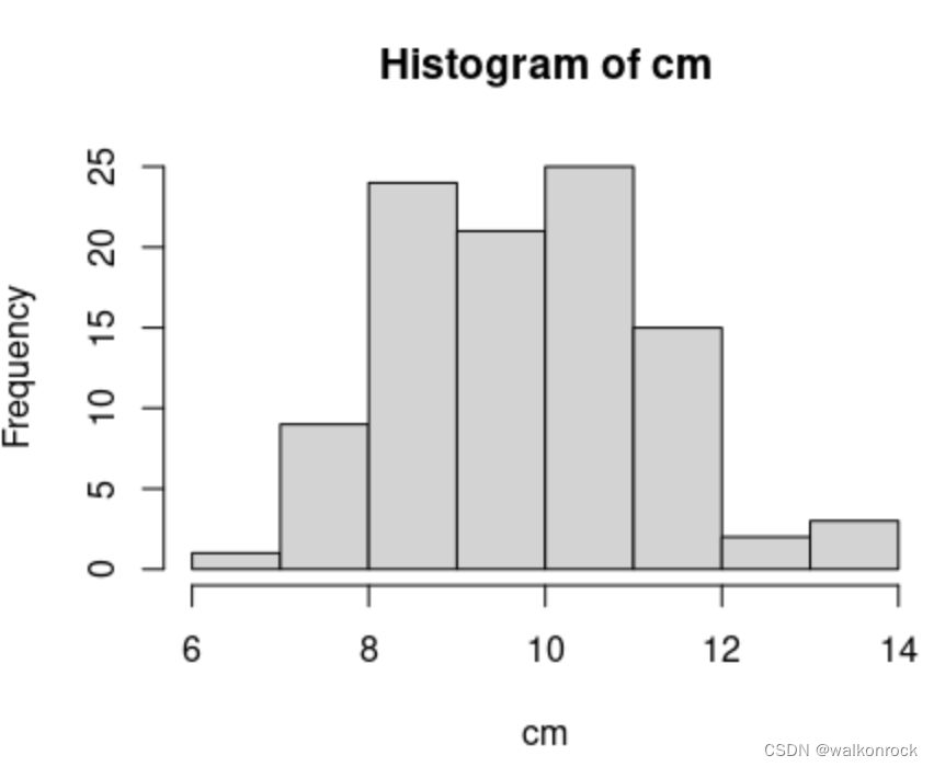
> cm <- colMeans(my_pois)
> hist(cm)

14. Base Graphics

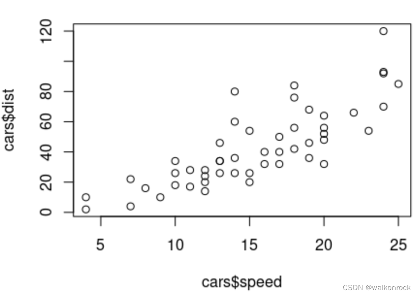
> data(cars)
> help(cars)
> head(cars)
  speed dist
1     4    2
2     4   10
3     7    4
4     7   22
5     8   16
6     9   10
> plot(cars)

> help(plot)
> plot(x = cars$speed, y = cars$dist)

> plot(x = cars$speed, y = cars$dist, xlab = "Speed") #x-axis set to "Speed"
> plot(x = cars$speed, y = cars$dist, ylab = "Stopping Distance") # y-axis set to "Stopping Distance"
> plot(cars, main="My Plot") # Plot cars with a main title of "My Plot"
> plot(cars,sub = "My Plot Subtitle") # Plot cars with a sub title of "My Plot Subtitle"
> plot(cars, col=2) # Plot cars so that the plotted points are colored red
> plot(cars, xlim=c(10, 15)) # Plot cars while limiting the x-axis to 10 through 15
> plot(cars, pch = 2) # Plot cars using triangles

boxplot(), like many R functions, also takes a “formula” argument, generally an expression with a tilde (“~”) which indicates the relationship between the input variables. This allows you to enter something like mpg ~ cyl to plot the relationship between cyl (number of cylinders) on the x-axis and mpg (miles per gallon) on the y-axis.

> boxplot(formula=mpg~cyl, data = mtcars)
> hist(mtcars$mpg)