


现在我们有了物体和每个像素多条射线,我们可以创建一些逼真的材质。我们将从漫反射材质(也称为哑光材质)开始。一个问题是我们是否混合和匹配几何体和材质(这样我们可以给多个球体分配相同的材质,或者反过来),还是几何体和材质是紧密关联的(这对于几何对象和材质链接的过程化对象可能会有用)。我们将选择分开处理,这在大多数渲染器中是常见的做法,但请注意还有其他替代方法。
9.1 A Simple Diffuse Material
不发光的散射物体仅仅会呈现出其周围环境的颜色,但是它们会通过自身的固有颜色来调节。反射在散射表面上的光线方向是随机的,因此,如果我们将三束光线发送到两个散射表面之间的缝隙中,它们会表现出不同的随机行为: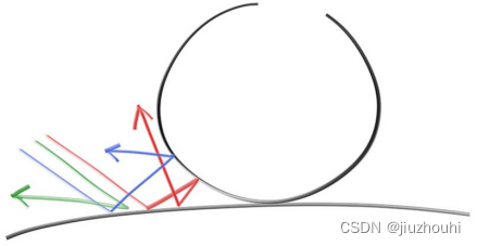
Figure 9: 光线的反射
它们也可能被吸收而非反射。表面越暗,光线被吸收的可能性就越大(这就是为什么它是暗的!)。实际上,任何随机改变方向的算法都会产生看起来呈哑光效果的表面。让我们从最直观的开始:一个随机将光线平等地向所有方向反射的表面。对于这种材质,击中表面的光线具有同等的概率以任意方向远离表面反射。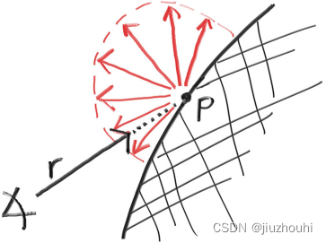
Figure 10: 地平线以上的等反射
这种非常直观的材质是最简单的漫反射材质,事实上,许多最早的光线追踪论文使用了这种漫反射方法(在采用稍后将要实现的更精确方法之前)。我们目前还没有一种随机反射光线的方法,因此我们需要在向量工具头文件中添加一些函数。我们首先需要的是生成任意随机向量的能力:
class vec3 {
  public:
...
    double length_squared() const {
        return e[0]*e[0] + e[1]*e[1] + e[2]*e[2];
    }
    static vec3 random() {
        return vec3(random_double(), random_double(), random_double());
    }
    static vec3 random(double min, double max) {
        return vec3(random_double(min,max), random_double(min,max),
random_double(min,max));
    }
};
然后我们需要找到一种方法来操作随机向量,以便只得到位于半球表面上的结果。有一些分析方法可以做到这一点,但实际上它们非常复杂,理解起来相当困难,并且实现起来也相当复杂。相反,我们将使用通常最简单的算法:拒绝采样法。拒绝采样法通过重复生成随机样本,直到满足所需的条件为止。换句话说,一直拒绝样本,直到找到一个好的样本。
使用拒绝采样法可以以许多等效有效的方式生成位于半球上的随机向量,但为了我们的目的,我们将选择最简单的方法:
1. 生成单位球内的随机向量。
2. 对该向量进行归一化。
3. 如果归一化后的向量位于错误的半球上,则反转该向量。
首先,我们将使用拒绝采样法生成单位球内的随机向量。从单位立方体中随机选择一个点,其中x、y和z的范围都是-1到+1,如果该点位于单位球外,则拒绝该点。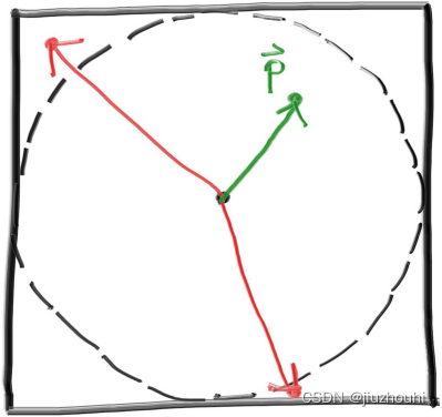
Figure 11: Two vectors were rejected before finding a good one
...
inline vec3 unit_vector(vec3 v) {
return v / v.length();
}

inline vec3 random_in_unit_sphere() {
while (true) {
auto p = vec3::random(-1,1);
if (p.length_squared() < 1)
    return p;
}
}
Listing 43: [vec3.h] The random_in_unit_sphere() function
一旦我们在单位球中获得一个随机向量,我们需要对其进行归一化,以获得一个单位球上的向量。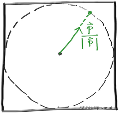
Figure 12: The accepted random vector is normalized to produce a unit vector
...
inline vec3 random_in_unit_sphere() {
while (true) {
        auto p = vec3::random(-1,1);
        if (p.length_squared() < 1)
            return p;
  }
}

inline vec3 random_unit_vector() {
return unit_vector(random_in_unit_sphere());
}
Listing 44: [vec3.h] Random vector on the unit sphere
既然我们在单位球的表面上有一个随机向量,我们可以通过将其与表面法线进行比较来确定它是否位于正确的半球上: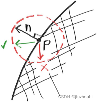
Figure 13: The normal vector tells us which hemisphere we need
我们可以对表面法线和随机向量进行内积,以确定它是否位于正确的半球上。如果内积为正数,则表示向量位于正确的半球上。如果内积为负数,则需要将向量反转。
...
inline vec3 random_unit_vector() {
return unit_vector(random_in_unit_sphere());
}

inline vec3 random_on_hemisphere(const vec3& normal) {
vec3 on_unit_sphere = random_unit_vector();
    if (dot(on_unit_sphere, normal) > 0.0) // In the same hemisphere as the normal
        return on_unit_sphere;
    else
        return -on_unit_sphere;
}
Listing 45: [vec3.h] The random_in_hemisphere() function
如果光线从材质上反射出来并完全保持其颜色,我们称该材质为白色。如果光线从材质上反射出来并完全失去其颜色,我们称该材质为黑色。作为对新的漫反射材质的第一个演示,我们将设置ray_color函数返回从反射中获得颜色的50%。我们应该期望得到一个不错的灰色。
class camera {
  ...
  private:
...
    color ray_color(const ray& r, const hittable& world) const {
        hit_record rec;
        if (world.hit(r, interval(0, infinity), rec)) {
            vec3 direction = random_on_hemisphere(rec.normal);
            return 0.5 * ray_color(ray(rec.p, direction), world);
        }
        vec3 unit_direction = unit_vector(r.direction());
        auto a = 0.5*(unit_direction.y() + 1.0);
        return (1.0-a)*color(1.0, 1.0, 1.0) + a*color(0.5, 0.7, 1.0);
    }
};
Listing 46: [camera.h] ray_color() using a random ray direction
...确实我们得到了非常漂亮的灰色球体: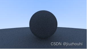
Image 7: First render of a diffuse sphere
9.2 Limiting the Number of Child Rays(限制子光线的数量)
这里存在一个潜在的问题。请注意,ray_color函数是递归的。何时停止递归呢?当它未能击中任何物体时停止。然而,在某些情况下,这可能需要很长时间,足以导致堆栈溢出。为了防止这种情况发生,让我们限制最大递归深度,在达到最大深度时不返回任何光照贡献。
class camera {
  public:
double aspect_ratio      = 1.0;  // Ratio of image width over height
int    image_width        = 100;  // Rendered image width in pixel count
int    samples_per_pixel = 10;   // Count of random samples for each pixel
int    max_depth         = 10;   // Maximum number of ray bounces into scene

void render(const hittable& world) {
    initialize();
    std::cout << "P3\n" << image_width << ' ' << image_height << "\n255\n";
    for (int j = 0; j < image_height; ++j) {
      std::clog <<"\rScanlines remaining: "<<(image_height - j)<<' '<< std::flush;
        for (int i = 0; i < image_width; ++i) {
           color pixel_color(0,0,0);
           for (int sample = 0;sample<samples_per_pixel;++sample){
             ray r = get_ray(i, j);
               pixel_color += ray_color(r, max_depth, world);
                }
                write_color(std::cout,pixel_color,samples_per_pixel);
            }
        }
        std::clog << "\rDone.                 \n";
    }
...
private:
    ...
    color ray_color(const ray& r, int depth, const hittable& world) const {
        hit_record rec;
        // If we've exceeded the ray bounce limit, no more light is gathered.
        if (depth <= 0)
            return color(0,0,0);
        if (world.hit(r, interval(0, infinity), rec)) {
            vec3 direction = random_on_hemisphere(rec.normal);
            return 0.5 * ray_color(ray(rec.p, direction), depth-1, world);
        }
       vec3 unit_direction = unit_vector(r.direction());
       auto a = 0.5*(unit_direction.y() + 1.0);
       return (1.0-a)*color(1.0, 1.0, 1.0) + a*color(0.5, 0.7, 1.0);
}
};
Listing 47: [camera.h] camera::ray_color() with depth limiting
更新main()函数以使用这个新的深度限制:
int main() {
...
camera cam;
cam.aspect_ratio      = 16.0 / 9.0;
cam.image_width       = 400;
cam.samples_per_pixel = 100;
cam.max_depth         = 50;
cam.render(world);
}
Listing 48: [main.cc] Using the new ray depth limiting
对于这个非常简单的场景,我们应该得到基本相同的结果: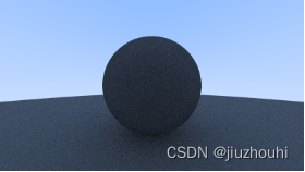
Image 8: Second render of a diffuse sphere with limited bounces
9.3 Fixing Shadow Acne(修复阴影粉刺)
还有一个需要解决的微小错误。当射线与表面相交时,射线会试图准确计算交点。不幸的是,这个计算容易受到浮点舍入误差的影响,导致交点略微偏离。这意味着下一条射线的起点,也就是从表面上随机散射出去的射线,可能与表面并不完全相切。它可能略高于表面,也可能略低于表面。如果射线的起点略低于表面,那么它可能再次与该表面相交。这意味着它会在 t=0.00000001 或其他浮点近似值处找到最近的表面,这是命中函数给出的结果。解决这个问题最简单的方法就是忽略非常接近计算交点的交点。
class camera {
  ...
  private:
...
color ray_color(const ray& r, int depth, const hittable& world) const{
   hit_record rec;
   // If we've exceeded the ray bounce limit, no more light is gathered.
   if (depth <= 0)
       return color(0,0,0);
       if (world.hit(r, interval(0.001, infinity), rec)) {
           vec3 direction = random_on_hemisphere(rec.normal);
           return 0.5 * ray_color(ray(rec.p, direction), depth-1, world);
     }
     vec3 unit_direction = unit_vector(r.direction());
     auto a = 0.5*(unit_direction.y() + 1.0);
     return (1.0-a)*color(1.0, 1.0, 1.0) + a*color(0.5, 0.7, 1.0);
}
};
Listing 49: [camera.h] Calculating reflected ray origins with tolerance
这样就解决了Shadow Acne。以下是结果: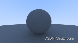
9.4 True Lambertian Reflection(真实的兰伯特反射)
将反射光线均匀地散射在半球上,可以产生一个漂亮的柔和散射模型,但我们肯定可以做得更好。对真实的漫反射物体的更准确表示是兰伯特分布。这个分布以与表面法线之间的角度cos(ϕ)成比例的方式散射反射光线。这意味着反射光线最有可能在接近表面法线的方向散射,并且在远离法线的方向散射的可能性较小。相比于之前的均匀散射,这种非均匀的兰伯特分布更好地模拟了真实世界材料的反射性能。
我们可以通过将一个随机单位向量添加到法线向量上来创建这个分布。在表面的交点上,有一个击中点p和一个表面的法线n。在交点处,这个表面有两个完全不同的面,因此任何交点只能有两个唯一的与之相切的单位球(一个单位球对应于表面的每个面)。这两个单位球将被其半径的长度位移离开表面,对于单位球来说,其半径的长度正好为1。
一个球将被位移朝着表面的法线(n)的方向,另一个球将被位移朝着相反的方向(−n)。这样,我们得到了两个单位大小的球,它们只会在交点处与表面接触。其中一个球的中心位于(P+n),而另一个球的中心位于(P−n)。中心在(P−n)处的球被认为在表面内部,而中心在(P+n)处的球被认为在表面外部。
我们希望选择与光线起点处于同一侧的切线单位球。在这个单位半径球上选择一个随机点S,并从击中点P发出一条光线指向随机点S(即向量(S−P))。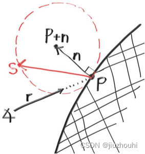
Figure 14: Randomly generating a vector according to Lambertian distribution
实际上,这个改变是相当小的:
class camera {
...
color ray_color(const ray& r, int depth, const hittable& world) const{
        hit_record rec;

        // If we've exceeded the ray bounce limit, no more light is gathered.
       if (depth <= 0)
            return color(0,0,0);

        if (world.hit(r, interval(0.001, infinity), rec)) {
            vec3 direction = rec.normal + random_unit_vector();
            return 0.5 * ray_color(ray(rec.p, direction), depth-1, world);
 	}
	vec3 unit_direction = unit_vector(r.direction());
 	auto a = 0.5*(unit_direction.y() + 1.0);
 	return (1.0-a)*color(1.0, 1.0, 1.0) + a*color(0.5, 0.7, 1.0);
}

};
Listing 50: [camera.h] ray_color() with replacement diffuse
渲染后,我们得到了一张相似的图像: 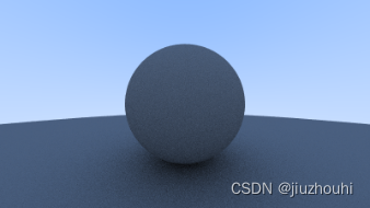
Image 10: Correct rendering of Lambertian spheres
在这两种漫反射方法中很难分辨出区别,因为我们的场景只包含两个简单的球体,但你应该能够注意到两个重要的视觉差异:
1. 改变后,阴影更加明显。
2. 改变后,两个球体都从天空中呈现出蓝色的色调。
这些变化都是由于光线的散射不均匀所造成的——更多的光线向法线方向散射。这意味着对于漫反射物体来说,它们会显得更暗,因为更少的光线反射到相机上。对于阴影来说,更多的光线会直接反射到上方,所以球体下面的区域会更暗。
日常生活中很少有完全漫反射的常见物体,因此我们对这些物体在光线下的行为的直观理解可能并不准确。随着本书中场景的复杂化,建议您在这里介绍的不同漫反射渲染器之间进行切换。大多数感兴趣的场景都会包含大量的漫反射材料。通过理解不同漫反射方法对场景照明的影响,您可以获得有价值的洞察。
9.5 使用伽马校正以获得准确的颜色强度
请注意球体下的阴影。图片非常暗,但是我们的球体只吸收每次反射的能量的一半,因此它们是50%的反射体。球体应该看起来相当亮(在现实生活中是浅灰色),但它们看起来相当暗淡。如果我们在漫反射材质上进行全亮度范围的遍历,我们可以更清楚地看到这一点。我们首先将ray_color函数的反射率从0.5(50%)设置为0.1(10%):
class camera {
...
color ray_color(const ray& r, int depth, const hittable& world) const {
     hit_record rec;

     // If we've exceeded the ray bounce limit, no more light is gathered.
     if (depth <= 0)
        return color(0,0,0);

     if (world.hit(r, interval(0.001, infinity), rec)) {
         vec3 direction = rec.normal + random_unit_vector();
         return 0.1 * ray_color(ray(rec.p, direction), depth-1, world);
     }
     vec3 unit_direction = unit_vector(r.direction());
     auto a = 0.5*(unit_direction.y() + 1.0);
     return (1.0-a)*color(1.0, 1.0, 1.0) + a*color(0.5, 0.7, 1.0);
}
};
Listing 51: [camera.h] ray_color() with 10% reflectance
我们以这个新的10%反射率进行渲染。然后我们将反射率设置为30%,再次进行渲染。我们依次重复50%、70%和最后90%的设置。您可以在所选的图片编辑器中从左到右叠加这些图像,您应该能够得到一个非常好的视觉表现,显示您选择的亮度范围逐渐增加。这是我们迄今为止一直在使用的那个: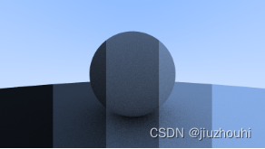
Image 11: The gamut of our renderer so far
仔细观察或使用取色器工具,您会注意到50%的反射率渲染图(位于中间)比起处于白色和黑色(中灰)中间位置的亮度要暗得多。事实上,70%反射率更接近中灰色。这是因为几乎所有的计算机程序在将图像写入图像文件之前都会假设该图像经过了“伽马校正”。这意味着0到1之间的值在存储为字节之前会应用一些变换。没有经过转换而直接写入数据的图像被称为处于线性空间,而经过转换的图像则被称为处于伽马空间。您使用的图像查看器可能期望接收的是伽马空间中的图像,而我们提供的是线性空间中的图像,这就是为什么我们的图像看起来过于暗淡的原因。
图像存储在伽马空间中有很多好处,但对于我们的目的,我们只需要意识到这一点即可。我们将把数据转换为伽马空间,以便我们的图像查看器可以更准确地显示图像。作为一个简单的近似,我们可以使用“gamma 2”作为我们的转换,这是从伽马空间到线性空间的转换所使用的幂次。我们需要从线性空间转换到伽马空间,这意味着取“gamma 2”的倒数,也就是指数为1/gamma,即平方根。
inline double linear_to_gamma(double linear_component){
return sqrt(linear_component);
}

void write_color(std::ostream &out, color pixel_color, int samples_per_pixel){
   auto r = pixel_color.x();
   auto g = pixel_color.y();
   auto b = pixel_color.z();

// Divide the color by the number of samples.
   auto scale = 1.0 / samples_per_pixel;
   r *= scale;
   g *= scale;
   b *= scale;

   // Apply the linear to gamma transform.
   r = linear_to_gamma(r);
   g = linear_to_gamma(g);
   b = linear_to_gamma(b);

   // Write the translated [0,255] value of each color component.
   static const interval intensity(0.000, 0.999);
  out << static_cast<int>(256 * intensity.clamp(r))
<< ' '<< static_cast<int>(256 * intensity.clamp(g))
    << ' '<< static_cast<int>(256 * intensity.clamp(b))
    << '\n';
}
Listing 52: [color.h] write_color(), with gamma correction
使用这种伽马校正,我们现在得到了一个更加一致的从暗到亮的渐变: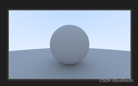


 1052
1052

 被折叠的 条评论
为什么被折叠?
被折叠的 条评论
为什么被折叠?
 到【灌水乐园】发言


