


文章目录
Pandas库
提供高性能易用数据类型和分析工具。
基于NumPy的扩展库,主要为了应用数据,主要强调了数据和索引之间的关系
import pandas as pd
Pandas主要提供两个数据类型:
- Series:一维数据类型
- DataFrame:二维至多维数据类型
及基于上述数据类型的各类操作。
Series类型
>>> import pandas as pd
>>> d = pd.Series(range(20))
>>> d
0      0
1      1
2      2
3      3
4      4
5      5
6      6
7      7
8      8
9      9
10    10
11    11
12    12
13    13
14    14
15    15
16    16
17    17
18    18
19    19
dtype: int64
>>> d.cumsum()
0       0
1       1
2       3
3       6
4      10
5      15
6      21
7      28
8      36
9      45
10     55
11     66
12     78
13     91
14    105
15    120
16    136
17    153
18    171
19    190
dtype: int64
左边是pandas为数据自动增加的索引,右边是值,类型为int64。
手动索引:
>>> b = pd.Series([9, 8, 7, 6], index=['a', 'b', 'c', 'd']) # 索引列表在第二个参数位时,可以省略index=,直接使用索引列表
>>> b
a    9
b    8
c    7
d    6
dtype: int64
生成和创建Series类型
>>> s = pd.Series(25, ['a', 'b', 'c']) # 标量创建
>>> s
a    25
b    25
c    25
dtype: int64
>>> d = pd.Series({'a':19, 'b':8, 'c':27}) # 字典创建
>>> d
a    19
b     8
c    27
dtype: int64
>>> e = pd.Series(({'a':19, 'b':8, 'c':27}), index=['c', 'a', 'b', 'd']) # 自定义字典结构
>>> e
c    27.0
a    19.0
b     8.0
d     NaN
dtype: float64
>>> import numpy as np
>>> n = pd.Series(np.arange(5)) # 使用ndarray生成
>>> n
0    0
1    1
2    2
3    3
4    4
dtype: int32
Series基本操作
>>> b
a    9
b    8
c    7
d    6
dtype: int64
>>> b.index # Series内部建立的类型
Index(['a', 'b', 'c', 'd'], dtype='object')
>>> b.values
array([9, 8, 7, 6], dtype=int64)
>>> b['b']
8
>>> b[1] # 即使指定索引,自动索引仍然存在
8
# b[['c', 'd', 0]] 目前已经不再支持这种混合使用的用法
>>> b[['c', 'd', 'a']]
c    7
d    6
a    9
dtype: int64
NumPy中的运算和操作可用于Series类型
>>> b[3]
6
>>> b[:3]
a    9
b    8
c    7
dtype: int64
>>> b[b>b.median()]
a    9
b    8
dtype: int64
>>> np.exp(b)
a    8103.083928
b    2980.957987
c    1096.633158
d     403.428793
dtype: float64
可使用字典的in和get等方法
>>> 'c' in b # in用于判断'c'是否在字典的键中
True
>>> 0 in b # 不会判断自动索引
False
>>> b.get('f', 100)
100
Series类型对齐操作
>>> a = pd.Series([1, 2, 3], ['c', 'd', 'e'])
>>> b
a    9
b    8
c    7
d    6
dtype: int64
>>> a
c    1
d    2
e    3
dtype: int64
>>> a + b # 加数中只有一个有值时,得出相应的结果位空
a    NaN
b    NaN
c    8.0
d    8.0
e    NaN
dtype: float64
Series类型的name属性
Series对象和索引都有一个名字,存储在属性.name中
>>> b.name
>>> b.name = 'Series对象'
>>> b.index.name = '索引列'
>>> b
索引列
a    9
b    8
c    7
d    6
Name: Series对象, dtype: int64
Series类型的修改
可随时修改并立即生效
>>> b['b', 'c'] = 20
>>> b
索引列
a     9
b    20
c    20
d     6
Name: Series对象, dtype: int64
DataFrame类型
DataFrame类型由共用相同索引的一组列组成。
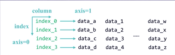
index为行索引,column为列索引
DataFrame创建
>>> import pandas as pd
>>> import numpy as np
>>> d = pd.DataFrame(np.arange(10).reshape(2, 5))  # 从二维ndarray对象创建
>>> d
   0  1  2  3  4
0  0  1  2  3  4
1  5  6  7  8  9
>>> dt = {'one':pd.Series([1, 2, 3], index=['a', 'b', 'c']),'two':pd.Series([9, 8, 7, 6], index=['a', 'b', 'c', 'd'])}
>>> d = pd.DataFrame(dt) # 从字典创建
>>> d
   one  two
a  1.0    9
b  2.0    8
c  3.0    7
d  NaN    6
>>> pd.DataFrame(dt, index=['b', 'c', 'd'], columns=['two', 'three'])
   two three
b    8   NaN
c    7   NaN
d    6   NaN
>>> dl = {'one':[1, 2, 3, 4], 'two':[9, 8, 7, 6]}
>>> d = pd.DataFrame(dl, index = ['a', 'b', 'c', 'd']) # 从列表类型字典创建
>>> d
   one  two
a    1    9
b    2    8
c    3    7
d    4    6
DataFrame每一列是一个Series对象。
Pandas数据类型操作
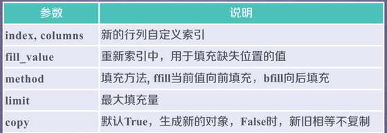
- .reindex():重新索引,重新排列Series和DataFrame索引如:d.reindex(columns=[‘a’, ‘b’, ‘c’])
.reindex(inedx=None, columns=None,…)
索引类型常用方法:
此处索引类型特指Pandas数据类型的索引,是一个不可修改的类型

Pandas库的数据类型运算
- 算术运算:根据行列索引,补齐后运算,运算默认产生浮点数,补齐时缺项默认为NaN(空值)。高维度和低维度之间为广播运算,如一维和零维进行运算,即一个数组和一个数,则这个数会和数组中的每个元素进行相加。采用加减乘除等符号时会产生新的对象。
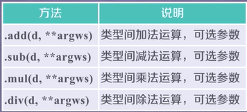
使用方法可以添加参数进行额外的操作,如添加fill_value参数代替NaN填补缺项 - 比较运算:只能比较相同索引对象,不进行补齐,高维和低维间进行广播运算,产生布尔对象
Pandas数据特征分析
排序
.sort_index():在指定轴上根据索引进行排序,默认升序
.sort_index(axis=0, ascending=True)
>>> sss = pd.DataFrame(np.arange(24).reshape(3, 8), index=['c', 'a', 'b'])
>>> sss
    0   1   2   3   4   5   6   7
c   0   1   2   3   4   5   6   7
a   8   9  10  11  12  13  14  15
b  16  17  18  19  20  21  22  23
>>> sss.sort_index()
    0   1   2   3   4   5   6   7
a   8   9  10  11  12  13  14  15
b  16  17  18  19  20  21  22  23
c   0   1   2   3   4   5   6   7
>>> sss.sort_index(ascending=False) # 降序排列
    0   1   2   3   4   5   6   7
c   0   1   2   3   4   5   6   7
b  16  17  18  19  20  21  22  23
a   8   9  10  11  12  13  14  15
>>> sss.sort_index(axis=1, ascending=False) # 对1轴排序
    7   6   5   4   3   2   1   0
c   7   6   5   4   3   2   1   0
a  15  14  13  12  11  10   9   8
b  23  22  21  20  19  18  17  16
.sort_values():在指定轴上根据数值排序,默认升序。 # 只是根据值对相应的行或列进行排序
Series.sort_values(axis=0, ascending=True)
DataFrame.sort_values(by, axis=0, ascending=True) by:axis轴上的某个索引或索引列表
>>> sss.sort_values(3, ascending=False) # 0轴默认为纵向
    0   1   2   3   4   5   6   7
b  16  17  18  19  20  21  22  23
a   8   9  10  11  12  13  14  15
c   0   1   2   3   4   5   6   7
>>> sss.sort_values('a', axis=1, ascending=False)
    7   6   5   4   3   2   1   0
c   7   6   5   4   3   2   1   0
a  15  14  13  12  11  10   9   8
b  23  22  21  20  19  18  17  16
NaN统一放在排序末尾,想让NaN参与排序,则可以将其替换再进行排序
统计分析
适用于Series类型和DataFrame类型:


>>> sss
    0   1   2   3   4   5   6   7
c   0   1   2   3   4   5   6   7
a   8   9  10  11  12  13  14  15
b  16  17  18  19  20  21  22  23
>>> sss.describe()
          0     1     2     3     4     5     6     7
count   3.0   3.0   3.0   3.0   3.0   3.0   3.0   3.0
mean    8.0   9.0  10.0  11.0  12.0  13.0  14.0  15.0
std     8.0   8.0   8.0   8.0   8.0   8.0   8.0   8.0
min     0.0   1.0   2.0   3.0   4.0   5.0   6.0   7.0
25%     4.0   5.0   6.0   7.0   8.0   9.0  10.0  11.0
50%     8.0   9.0  10.0  11.0  12.0  13.0  14.0  15.0
75%    12.0  13.0  14.0  15.0  16.0  17.0  18.0  19.0
max    16.0  17.0  18.0  19.0  20.0  21.0  22.0  23.0
>>> type(sss.describe())
<class 'pandas.core.frame.DataFrame'>
>>> sss.describe().loc['max'] # 对Series对象不需要用loc
0    16.0
1    17.0
2    18.0
3    19.0
4    20.0
5    21.0
6    22.0
7    23.0
Name: max, dtype: float64
在1.0之后的pandas版本中,ix已经被废弃,只能使用loc和iloc
对于loc和iloc的区别见:
https://blog.csdn.net/sushangchun/article/details/83514803
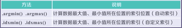
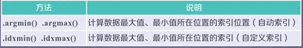
只适用于Series类型:
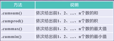
数据的累计统计分析
适用于Series和DataFrame类型:
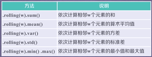
滚动计算(窗口计算)函数:
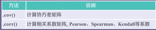
数据的相关性分析
- 利用协方差描述
- 利用Pearson相关系数
两个事物表现为X和Y
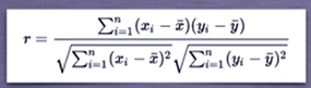
r取值范围为[-1, 1] - 0.8-1.0为极强相关
- 0.6-0.8为强相关
- 0.4-0.6为中等强度相关
- 0.2-0.4弱相关
- 0.0-0.2极弱相关或无关
>>> hprice = pd.Series([3.04, 22.93, 12.75, 22.6, 12.33], index=['2008', '2009', '2010', '2011', '2012'])
>>> hprice
2008     3.04
2009    22.93
2010    12.75
2011    22.60
2012    12.33
dtype: float64
>>> m2 = pd.Series([8.18, 18.38, 9.13, 7.82, 6.69], index=['2008', '2009', '2010', '2011', '2012'])
>>> m2
2008     8.18
2009    18.38
2010     9.13
2011     7.82
2012     6.69
dtype: float64
>>> hprice.corr(m2)
0.5239439145220387
>>> import matplotlib.pyplot as plt
>>> plt.plot(hprice)
[<matplotlib.lines.Line2D object at 0x000001B0468F7490>]
>>> plt.plot(m2)
[<matplotlib.lines.Line2D object at 0x000001B0468F7790>]
>>> plt.show()


 551
551


 被折叠的 条评论
为什么被折叠?
被折叠的 条评论
为什么被折叠?
 到【灌水乐园】发言


