贪婪迭代法解决流水车间调度问题

jqgogogo

已于 2022-05-21 19:26:18 修改

阅读量1.9k

点赞数 8

文章标签：算法 matlab

于 2022-05-20 19:54:19 首次发布

本文链接：https://blog.csdn.net/jqgogogo/article/details/124886937

版权

最近导师问我有没有matlab关于一些简单的规模调度问题的代码，我没用过matlab所以就准备在网上找一个，看了以下大部分都是不全的，要么就是要收费的。就在网上参考了一篇2018年GECCO的论文Iterated greedy algorithms for the hybrid flowshop scheduling with total flow time minimization。这篇论文研究的是混合流水车间调度问题，采用一种新的贪婪迭代方法求解。因为混合车间调度问题考虑起来有点复杂，为了快点做完交给老师，我把问题改成了流水车间调度问题，花了一天的时间实现了原文算法的大部分内容，因为我的问题比较简单规模也比较小，所以没必要实现全部内容。下面就分析一下原文中的算法，并给出我实现的完整代码，方便有需要的人学习。关于流水车间调度问题的模型和介绍，网上资源有而且也比较详细，我就不多写了。

算法流程

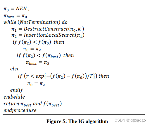
这个是原文中算法的主体流程，主要部分包括NEH生成初始解、destructconstruct破坏和生成、insertionLocalSearch插入局部搜索、更新最优解这四部分组成。

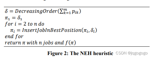
NEH生成初始解

NEH生成初始解在原文的参考文献中有，不懂可以去看参考文献，写的十分详细。

% 初始化加工序列
% 采用NEH初始化方法
function ret = neh(process_time)
[nb_jobs,~] = size(process_time); % 工件数和阶段数
sum_time = sum(process_time,2); % 求出总加工时间
[~,index] = sort(sum_time); % 返回排序后的索引
pre=index(1);% pre表示前面部分
next=index(2:nb_jobs); % next表示要插入的所有工件
len=length(next);
for i=1:len
    pre=InsertBestPostion(pre,next(i),process_time); % 将next(i)插入pre所有可能的位置,返回最佳序列
end
ret=pre;
end

InsertBestPosition

% 参数说明 seq：部分序列 job：待插入的工件 process_time:加工时间
% 在seq中找到最佳插入点插入job,返回插入后的seq
function ret=InsertBestPostion(seq,job,process_time)
len=length(seq);
for i=1:len+1
    if i==1
        new_seq=[job,seq(1:end)]; % 在seq前插入
    else
        new_seq=[seq(1:i-1),job,seq(i:end)]; % 在seq中插入
    end
    [ctime,~]=decode(new_seq,process_time); % 解码得到新的序列加工时间
    % 找出最优序列
    if i==1
       cbest=ctime;
       best_seq=new_seq;
    elseif i>1 && ctime<cbest
       cbest=ctime;
       best_seq=new_seq;
    end
end
    ret=best_seq;
end

Decode

decode负责对一个序列seq进行解码，得到seq的完工时间

% decode对seq进行解码 计算seq的完成时间
function [ctime,all]= decode(seq,process_time)
[jobs,machines]=size(process_time);
len = length(seq);
complete = zeros(jobs,machines); % 记录工件的完成时间
for m=1:machines
    for j=1:len
        number=seq(j);
        if m==1 && j==1
            % 第1个机器上的第1个工件,完成时间等于所需要的加工时间
            complete(number,m)=process_time(number,m); 
        elseif m == 1 && j>1
            % 第1个机器上加工次序大于1的工件 完成时间=前一工件的完成时间 + 所需时间
            complete(number,m)=process_time(number,m) + complete(last_number,m);
        elseif m>1 && j == 1
            % 第m个机器上第1个工件 完成时间 = 第1个工件在第m-1机器上的完工时间 + 所需时间
            complete(number,m)=complete(number,m-1) + process_time(number,m);
        else
            % 第m个机器上第j个工件 完成时间 = max(该工件在上一机器上的完成时间,当前机器上前一工件的完成时间) + 所需时间
            complete(number,m)=max(complete(number,m-1),complete(last_number,m)) + process_time(number,m);
        end
        last_number = number;
    end
end
ctime = complete(seq(len),machines); % 完工时间
all=complete;
end

DestructConstruct

该步骤分为两步：第1步破坏，即不重复的从解中随机选择k个工件作为插入元素，将解中这k个元素删除，得到部分序列。第2步构造，将k个元素依次插入部分解的最好位置，得到完整的序列。

% 拆分并构造新解返回最佳构造的解
function ret = destruct(seq,k,process_time)
len=length(seq);
insert=randperm(len,k); % 随机选择k个元素作为插入元素
for i=1:k
    index=seq==insert(i);
    seq(index)=[]; % seq中删除要插入的元素
end
for i=1:k
    seq=InsertBestPostion(seq,insert(i),process_time); % 找到seq的最佳插入位置得到新的seq
end
ret=seq;
end

localsearch

然后就是局部搜索，在论文中采用了两种局部搜索。第1步，First improvement insertion local search。第2步，RIS local search。下面依次介绍这两种局部搜索。

% 局部搜索
function ret=localsearch(seq,best_seq,process_time)
seq1=improvement(seq,process_time);
seq2=RISsearch(seq1,best_seq,process_time);
ret=seq2;
end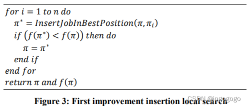

% 第1步局部搜索
function ret=improvement(seq,process_time)
len=length(seq);
old_ctime = decode(seq,process_time);
for i=1:len
    old_seq=seq;
    job=old_seq(i); % 插入元素
    old_seq(i)=[]; % 将插入元素移除
    new_seq=InsertBestPostion(old_seq,job,process_time); % 得到最佳插入序列
    [new_ctime,~]=decode(new_seq,process_time);
    if new_ctime < old_ctime
        old_ctime = new_ctime;
        seq = new_seq;
    end
end
ret=seq;
end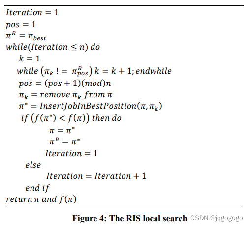

RIS局部搜索的主要思想是：将当前搜索到的最佳序列作为搜索方向的指导解。举个例子吧，一个序列代表5个工件的解seq=[1,2,3,4,5]，一个当前最优best=[5,1,4,3,2]，首先移除seq的工件5，然后将工件5插入到seq的所有可能位置，找到最佳插入位置的解new_seq，如果new_seq的完工时间小于seq，则将seq替换为new_seq，同时将计数器iter归1，否则iter+1。然后进入下一步，从seq中移除第2个工件1，插入seq的所有可能位置，找到最优插入位置的解...，重复这个过程直到iter大于len。

% 第2步局部搜索
function ret = RISsearch(seq,best_seq,process_time)
iter=1;
pos=1;
len=length(seq);
[old_ctime,~]=decode(seq,process_time);
while iter<=len
    k=1;
    while seq(k) ~= best_seq(pos) && k <=len
        k=k+1;
    end
    pos=mod(pos+1,len)+1;
    old_seq=seq;
    job=old_seq(k);
    old_seq(k)=[];
    new_seq=InsertBestPostion(old_seq,job,process_time);
    [new_ctime,~]=decode(new_seq,process_time);
    if new_ctime < old_ctime
        seq=new_seq;
        old_ctime=new_ctime;
        iter=1;
    else
        iter=iter+1;
    end
end
ret=seq;
end

FSP

介绍完了算法的所有模块，下面就给出主函数入口。代码和前面的函数流程是一致的，主要模块前面已经介绍了，就是借鉴了模拟退火的思想，当seq2比seq要差时，以概率以exp(-(f(seq2)-f(seq))/T)的概率接受seq2，T为参数论文中给出的公式是：

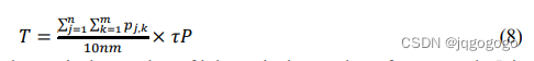
n为工件数、m为机器数，p（j，k）表示所需加工时间，作者给出后面那个参数取0.4，可以计算出T。

% 主函数入口
% 采用贪婪迭代方法搜索
% 参考论文 Iterated greedy algorithms for the hybrid flowshop scheduling with total flow time minimization 
% Hande Öztop M. Fatih Tasgetiren Deniz Türsel Eliiyi Quan-Ke Pan in GECCO 2018
function fsp
% 初始化数据
nb_jobs = 20; % 工件数
nb_machines = 10; % 机器数
process_time = randi([20,50],nb_jobs,nb_machines); % 加工时间
termination = 100; % 迭代次数
seq = neh(process_time); % 初始化序列
best_seq=seq; % 历史最优解
[best_ctime,~]=decode(best_seq,process_time);
k=2; % 重插入工件数量
tao=0.4; % 温度接受标准
T=sum(process_time,"all")*tao/(10*nb_jobs*nb_machines); % 模拟退火的温度
for i=1:termination
    seq1=destruct(seq,k,process_time); 
    seq2=localsearch(seq1,best_seq,process_time);
    [ctime1,~]=decode(seq,process_time);
    [ctime2,~]=decode(seq2,process_time);
    if ctime2<ctime1 % ctime2小于ctime1意味这seq2比seq更优
        seq=seq2; % 更新seq
        if ctime2<best_ctime
            best_seq=seq2; % 同样如果比best_seq更优则,更新best_seq
        end
    else
        r=rand(1);
        if r<exp(-(ctime2-ctime1)/T) % 以exp(-(f(seq2)-f(seq))/T)的概率接受seq2
            seq=seq2;
        end
    end
end
[~,time]=decode(best_seq,process_time);
draw(best_seq,time,process_time);
end

绘图部分

color1和color2分别代表两组颜色取值，color1一共有10种颜色，color2一共有20中颜色。所以工件数n不要超过20，否则就要添加更多的颜色类别。

function []=draw(seq,time,process_time)
clc;
[jobs,machines]=size(time);
xlabel("加工时间","FontSize",16,"FontWeight","bold");
set(gca,'ytick',0:1:machines);
ylabel("加工机器","FontSize",16,"FontWeight","bold");
txt=sprintf("完工时间=%d",time(seq(jobs),machines));
title(txt,"FontSize",16,"FontWeight","bold");
% 绘图所需颜色
color1 = [0.57, 0.69, 0.30;
         0.89, 0.88, 0.57;
         0.76, 0.49, 0.58;
         0.47, 0.76, 0.81;
         0.21, 0.21, 0.35;
         0.28, 0.57, 0.54;
         0.07, 0.35, 0.40;
         0.41, 0.20, 0.42;
         0.60, 0.24, 0.18;
         0.76, 0.84, 0.65];
color2= [0.77, 0.18, 0.78;
          0.21, 0.33, 0.64;
          0.88, 0.17, 0.56;
          0.20, 0.69, 0.28;
          0.26, 0.15, 0.47;
          0.83, 0.27, 0.44;
          0.87, 0.85, 0.42;
          0.85, 0.51, 0.87;
          0.99, 0.62, 0.76;
          0.52, 0.43, 0.87;
          0.00, 0.68, 0.92;
          0.26, 0.45, 0.77;
          0.98, 0.75, 0.00;   
          0.72, 0.81, 0.76;
          0.77, 0.18, 0.78;
          0.28, 0.39, 0.44;
          0.22, 0.26, 0.24;
          0.64, 0.52, 0.64;
          0.87, 0.73, 0.78;
          0.94, 0.89, 0.85;
          0.85, 0.84, 0.86];
for i=1:machines
    for j=1:jobs
        number=seq(j);
        ctime=time(number,i); %完成时间点
        need_time = process_time(number,i); %所需时间
        txt=sprintf("J%d",number);% 工件编号
        rec=[ctime-need_time,i-0.25,need_time,0.5]; %矩形框的大小和位置 [x,y,w,h]
        rectangle("Position",rec,'LineWidth',0.5,'LineStyle','-','FaceColor',color2(number,:)); % 绘制矩形
        text(ctime-need_time+0.5,i,txt,"FontSize",10,"FontWeight","bold"); % 绘制标注信息
    end
end
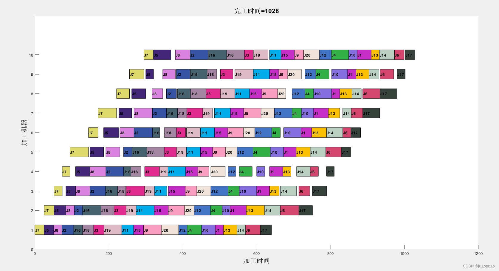
end

实验结果

绘制工件n=20，机器m=10的加工甘特图

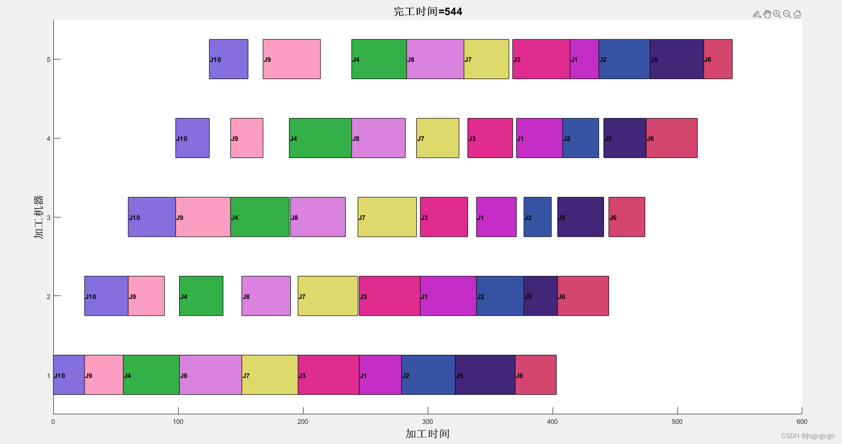
工件n=10，机器m=5的甘特图

jqgogogo

关注

8
点赞
踩
30

收藏

觉得还不错? 一键收藏
1
评论
贪婪迭代法解决流水车间调度问题

最近导师问我有没有matlab关于一些简单的规模调度问题的代码，我没用过matlab所以就准备在网上找一个，看了以下大部分都是不全的，要么就是要收费的。就在网上参考了一篇2018年GECCO的论文Iterated greedy algorithms for the hybrid flowshop scheduling with total flow time minimization。这篇论文研究的是混合流水车间调度问题，采用一种新的贪婪迭代方法求解。因为混合车间调度问题考虑起来有点复杂，为了快点做完交给老
复制链接

扫一扫