Tensorflow进行深度学习(第二)

进行mnist的入门教程

程序中下载安装mnist的数据，使用代码如下所示：下载地址

下载后进行加载‘MNIST_data’

import input_data
mnist = input_data.read_data_sets("MNIST_data/", one_hot=True)

运行tensorflow的InteractiveSession:

运行InteractiveSession类。通过它，你可以更加灵活的构建代码。它能让你在运算图的时候，插入一些计算图，这些计算图由简单的操作（operations）构成，如果不使用InteractiveSession，那么你需要在启动session之前构建整个计算图，然后启动该计算图。

sess = tf.InteractiveSession()

现在构建一个Softmax回归模型：线性的

占位符：

我们通过为输入图像和目标输出类别创建节点，来开始构建计算图。

x = tf.placeholder("float", shape=[None, 784])
y_ = tf.placeholder("float", shape=[None, 10])

x，y_是占位符

下面完整的代码：

# coding: UTF-8
import tensorflow as tf
import numpy as np
import matplotlib.pyplot as plt
import input_data


mnist = input_data.read_data_sets("MNIST_data/", one_hot=True)

training = mnist.train.images
trainlable = mnist.train.labels
testing = mnist.test.images
testlabel = mnist.test.labels

print ("MNIST loaded")

print(training.shape)
print (trainlable.shape)
print (testing.shape)
print (testlabel.shape)

sess = tf.InteractiveSession()
# 初始化变量
x = tf.placeholder("float", shape=[None, 784])
y_ = tf.placeholder("float", shape=[None, 10])
W = tf.Variable(tf.zeros([784, 10]))
b = tf.Variable(tf.zeros([10]))

sess.run(tf.initialize_all_variables())
y = tf.nn.softmax(tf.matmul(x, W) + b)
cross_entropy = -tf.reduce_sum(y_*tf.log(y))
train_step = tf.train.GradientDescentOptimizer(0.004).minimize(cross_entropy)
for i in range(2000):
  batch = mnist.train.next_batch(50)
  train_step.run(feed_dict={x: batch[0], y_: batch[1]})
correct_prediction = tf.equal(tf.argmax(y, 1), tf.argmax(y_, 1))

accuracy = tf.reduce_mean(tf.cast(correct_prediction, "float"))
print accuracy.eval(feed_dict={x: mnist.test.images, y_: mnist.test.labels})

先将x，y_占位符，W是权重，因为图片是28×28的，而且最后的形式是生成10个分类的效果，因为我们有784个特征和10个输出值。b是偏移量。然后在sess中进行全局变量的初始化。

y进行softmax运算，我们的损失函数是目标类别和预测类别之间的交叉熵。

cross_entropy = -tf.reduce_sum(y_*tf.log(y))

然后进行训练模型。

上面建立的是一个单层的简单神经网络，下面建立一个两层的简单的神经网络。

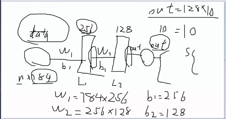
如图所示就是创建一个两层的神经网络，第一：data是输入的mnist数据集，大小是n*784，第二：然后就是权重w1 加上偏执 b1，经过第一层神经网络，我们设置第一层的神经网络的大小为256个神经元，则w1=784×256，b1=256

然后经过一个非线性的sigmod函数。第三：经过第二层的神经网络，设置大小为128个神经元，则w2=256×128，b2=128，然后经过一个非线性的sigmod函数。第四：经过out，则大小128×10，b=10

得到输出。

# coding = UTF-8

import tensorflow as tf
import numpy as np
import matplotlib.pyplot as plt
import input_data

# 引入mnist数据集
mnist = input_data.read_data_sets('data/', one_hot=True)

'''
network topologies 设置网络的拓扑结构,分别是隐藏层的大小，输入的大小，输出的大小
'''
n_hidden_1 = 256
n_hidden_2 = 128
n_input = 784
n_classes = 10
'''
设置输入和输出的占位，为下面计算时填充。
'''
# input and outputs
x = tf.placeholder("float", shape=[None, n_input])
y = tf.placeholder("float", shape=[None, n_classes])
'''
设置网络参数，分别是图中的权重参数，和偏执参数。
'''
# network parameters
stddev = 0.1
weights = {
    'w1': tf.Variable(tf.random_normal([n_input, n_hidden_1], stddev=stddev)),
    'w2': tf.Variable(tf.random_normal([n_hidden_1, n_hidden_2], stddev=stddev)),
    'out': tf.Variable(tf.random_normal([n_hidden_2, n_classes], stddev=stddev))
}
biase = {
    'b1': tf.Variable(tf.random_normal([n_hidden_1])),
    'b2': tf.Variable(tf.random_normal([n_hidden_2])),
    'out': tf.Variable(tf.random_normal([n_classes]))
}
print("network ready")

'''
进行前置传播函数
'''
def multilay_perceptron(_X, _weights, _biases):
    layer_1 = tf.nn.sigmoid(tf.add(tf.matmul(_X, _weights['w1']), _biases['b1']))
    layer_2 = tf.nn.sigmoid(tf.add(tf.matmul(layer_1, _weights['w2']), _biases['b2']))
    return tf.matmul(layer_2, _weights['out']) + _biases['out']

'''
前置传播
'''
# prediction
pred = multilay_perceptron(x, weights, biase)
'''
损失函数和最优化
'''
# loss and optimizer
# reduce_mean 会求出/n，
cost = tf.reduce_mean(tf.nn.softmax_cross_entropy_with_logits(pred, y))
# 反向传播，梯度下降算法，求出最小的cost值
optm = tf.train.GradientDescentOptimizer(learning_rate=0.01).minimize(cost)
# 错误率的求
corr = tf.equal(tf.argmax(pred, 1), tf.argmax(y, 1))
# 正确率
accr = tf.reduce_mean(tf.cast(corr, "float"))


# initializer初始化全部的变量
init = tf.initialize_all_variables()
print ("function ready")

# 运算时的参数
training_epochs = 20
batch_size = 100
display_step = 4

# 生出图模型
# launch the graph
sess = tf.Session()
sess.run(init)

'''
进行模型的训练
'''
# optimize
for epoch in range(training_epochs):
    avg_cost = 0.
    total_batch = int(mnist.train.num_examples/batch_size)
    # iteration
    for i in range(total_batch):
        batch_xs, batch_ys = mnist.train.next_batch(batch_size)
        feeds = {x: batch_xs, y: batch_ys}
        sess.run(optm, feed_dict=feeds)
        avg_cost += sess.run(cost, feed_dict=feeds)
    avg_cost = avg_cost / total_batch
    # display显示每次epoch的训练的准确率和测试的准确率。
    if (epoch+1) % display_step == 0:
        print ("epoch: %03d%03d cost: %.9f" % (epoch, training_epochs,avg_cost))
        feeds = {x: batch_xs, y: batch_ys}
        train_acc = sess.run(accr, feed_dict=feeds)
        print ("TRAIN ACCURACY: %.3f" % (train_acc))
        feeds = {x: mnist.test.images, y: mnist.test.labels}
        test_acc = sess.run(accr, feed_dict=feeds)
        print ("TEST ACCURACY: %.3f" % (test_acc))
print ("optimization finished")

建立一个多层的卷积网络：

# coding: UTF-8
import tensorflow as tf
import numpy as np
import matplotlib.pyplot as plt
import input_data
'''
得到数据
'''
mnist = input_data.read_data_sets("MNIST_data/", one_hot=True)

training = mnist.train.images
trainlable = mnist.train.labels
testing = mnist.test.images
testlabel = mnist.test.labels

print ("MNIST loaded")
# 获取交互式的方式
sess = tf.InteractiveSession()
# 初始化变量
x = tf.placeholder("float", shape=[None, 784])
y_ = tf.placeholder("float", shape=[None, 10])
W = tf.Variable(tf.zeros([784, 10]))
b = tf.Variable(tf.zeros([10]))
'''
生成权重函数，其中shape是数据的形状
'''
def weight_variable(shape):
    initial = tf.truncated_normal(shape, stddev=0.1)
    return tf.Variable(initial)
'''
生成偏执项 其中shape是数据形状
'''
def bias_variable(shape):
    initial = tf.constant(0.1, shape=shape)
    return tf.Variable(initial)

def conv2d(x, W):
    return tf.nn.conv2d(x, W, strides=[1, 1, 1, 1], padding='SAME')

def max_pool_2x2(x):
    return tf.nn.max_pool(x, ksize=[1, 2, 2, 1],
                          strides=[1, 2, 2, 1], padding='SAME')

W_conv1 = weight_variable([5, 5, 1, 32])
b_conv1 = bias_variable([32])
x_image = tf.reshape(x, [-1, 28, 28, 1])

h_conv1 = tf.nn.relu(conv2d(x_image, W_conv1) + b_conv1)
h_pool1 = max_pool_2x2(h_conv1)

W_conv2 = weight_variable([5, 5, 32, 64])
b_conv2 = bias_variable([64])

h_conv2 = tf.nn.relu(conv2d(h_pool1, W_conv2) + b_conv2)
h_pool2 = max_pool_2x2(h_conv2)


W_fc1 = weight_variable([7 * 7 * 64, 1024])
b_fc1 = bias_variable([1024])

h_pool2_flat = tf.reshape(h_pool2, [-1, 7*7*64])
h_fc1 = tf.nn.relu(tf.matmul(h_pool2_flat, W_fc1) + b_fc1)

keep_prob = tf.placeholder("float")
h_fc1_drop = tf.nn.dropout(h_fc1, keep_prob)

W_fc2 = weight_variable([1024, 10])
b_fc2 = bias_variable([10])

y_conv=tf.nn.softmax(tf.matmul(h_fc1_drop, W_fc2) + b_fc2)

cross_entropy = -tf.reduce_sum(y_*tf.log(y_conv))
train_step = tf.train.AdamOptimizer(1e-4).minimize(cross_entropy)
correct_prediction = tf.equal(tf.argmax(y_conv, 1), tf.argmax(y_, 1))
accuracy = tf.reduce_mean(tf.cast(correct_prediction, "float"))
sess.run(tf.initialize_all_variables())
for i in range(20000):http://write.blog.csdn.net/postedit/72801694
  batch = mnist.train.next_batch(50)
  if i%100 == 0:
    train_accuracy = accuracy.eval(feed_dict={
        x:batch[0], y_: batch[1], keep_prob: 1.0})
    print "step %d, training accuracy %g"%(i, train_accuracy)
  train_step.run(feed_dict={x: batch[0], y_: batch[1], keep_prob: 0.5})

print "test accuracy %g"%accuracy.eval(feed_dict={
    x: mnist.test.images, y_: mnist.test.labels, keep_prob: 1.0})

另外一种两层的卷积神经网络：

# coding: UTF-8

import tensorflow as tf
import numpy as np
import input_data

mnist = input_data.read_data_sets("MNIST_data/", one_hot=True)
training = mnist.train.images
trainlable = mnist.train.labels
testing = mnist.test.images
testlabel = mnist.test.labels

print ('mnist loaded')

n_input = 784
n_output = 10
weights = {

    # tensorflow 做卷积的时候参数是四维的[3,3,1,64]，第一个代表filter的height，第二个参数weight，第三个参数代表连接输入深度（灰度为1），第四个参数代表
    # 输出的大小即output channel.

    'wc1': tf.Variable(tf.random_normal([3, 3, 1, 64], stddev=0.1)),
    'wc2': tf.Variable(tf.random_normal([3, 3, 64, 128], stddev=0.1)),

    # 全连接层，第一个参数为输入，第二个参数为输出。其中7×7×128,经过两层的max_pool最终减小为1/4.
    # 全连接层作用将第一个参数大小转换成第二个参数大小。比如7×7×128-->1024

    'wd1': tf.Variable(tf.random_normal([7*7*128, 1024], stddev=0.1)),
    'wd2': tf.Variable(tf.random_normal([1024, n_output], stddev=0.1))
}
biases = {

    # 偏移量中的参数，代表其中的大小。

    'bc1': tf.Variable(tf.random_normal([64], stddev=0.1)),
    'bc2': tf.Variable(tf.random_normal([128], stddev=0.1)),
    'bd1': tf.Variable(tf.random_normal([1024], stddev=0.1)),
    'bd2': tf.Variable(tf.random_normal([n_output], stddev=0.1))
}

# 进行卷积加池化的操作
def conv_basic(_input, _w, _b, _keepratio):

    # shape的参数[-1,28,28,1],其中第一个参数是batch的大小，若为-1则表示自动补全，
    # 第二个和第三个参数表示height和weight，最后个代表channel通道

    _input_r = tf.reshape(_input, shape=[-1, 28, 28, 1])

    #tf.nn.conv2d(input, filter, strides, padding,
    #use_cudnn_on_gpu=None, data_format=None, name=None)
    # 第一参数是输入，第二个参数是字典，
    # 第三个strides[1,1,1,1]，分别表示batch,height,wight,channel。
    # padding有两种形式，‘SAME’填充，'VALID'不填充。
    # tf.nn.max_pool(value, ksize, strides, padding, data_format='NHWC', name=None)

    _conv1 = tf.nn.conv2d(_input_r, _w['wc1'], strides=[1, 1, 1, 1], padding='SAME')
    _conv1 = tf.nn.relu(tf.nn.bias_add(_conv1, _b['bc1']))
    _pool1 = tf.nn.max_pool(_conv1, ksize=[1, 2, 2, 1], strides=[1, 2, 2, 1], padding='SAME')
    _pool_dr1 = tf.nn.dropout(_pool1, _keepratio)

    _conv2 = tf.nn.conv2d(_pool_dr1, _w['wc2'], strides=[1, 1, 1, 1], padding='SAME')
    _conv2 = tf.nn.relu(tf.nn.bias_add(_conv2, _b['bc2']))
    _pool2 = tf.nn.max_pool(_conv2, ksize=[1, 2, 2, 1], strides=[1, 2, 2, 1], padding='SAME')
    _pool_dr2 = tf.nn.dropout(_pool2, _keepratio)
    # VECTORIZE
    _densel = tf.reshape(_pool_dr2, [-1, 7*7*128])
    # 全连接层1
    _fc1 = tf.nn.relu(tf.add(tf.matmul(_densel, _w['wd1']), _b['bd1']))
    _fc_drl = tf.nn.dropout(_fc1, _keepratio)
    # 全连接层2
    _out = tf.add(tf.matmul(_fc_drl, _w['wd2']), _b['bd2'])
    # 返回
    out = {'input_r': _input_r, 'conv1': _conv1, 'pool1': _pool1,
           'pool1_dr1': _pool_dr1,
           'conv2': _conv2, 'pool2': _pool2,
           'pool_dr2': _pool_dr2,
           'densel': _densel,
           'fc1': _fc1,
           'fc_drl': _fc_drl,
           'out': _out
    }
    return out

print ("cnn ready")

x = tf.placeholder(tf.float32, [None, n_input])
y = tf.placeholder(tf.float32, [None, n_output])
keepratio = tf.placeholder(tf.float32)

# function
_pred = conv_basic(x, weights, biases, keepratio)['out']

cost = tf.reduce_mean(tf.nn.softmax_cross_entropy_with_logits(_pred, y))

optm = tf.train.AdamOptimizer(learning_rate=0.001).minimize(cost)
_corr = tf.equal(tf.argmax(_pred, 1), tf.argmax(y, 1))
accr = tf.reduce_mean(tf.cast(_corr, tf.float32))
init = tf.initialize_all_variables()

# saver
print("graph ready")

sess = tf.InteractiveSession()
sess.run(init)

training_epochs = 15
batch_size = 16
display_step = 1
for epoch in range(training_epochs):
    avg_cost = 0
    total_batch = 10
    for i in range(total_batch):
        batch_xs, batch_ys = mnist.train.next_batch(batch_size)
        keeps = {x: batch_xs, y: batch_ys, keepratio: 0.7}
        sess.run(optm, feed_dict=keeps)
        avg_cost += sess.run(cost, feed_dict={x: batch_xs, y: batch_ys, keepratio: 1.})/total_batch
    if epoch%display_step == 0:
        print ("epoch:%03d training_epochs:%03d  cost:%0.9f" % (epoch, training_epochs, avg_cost))
        train_acc = sess.run(accr, feed_dict={x:batch_xs, y:batch_ys, keepratio:1.})
        print("test accuracy:%.3f"%(train_acc))

print ("optimization finished")

其中代码的详细解释都在注释当中，代码运行的时候出现了一个类型不匹配的问题，经过查找发现是在进行池化的过程中ksize和strides的大小不一样导致的。因此池化过程需要ksize和strides的大小要一样。
 

保存运行中产生的model，即权重和偏置项。

# coding: "UTF-8"
import tensorflow as tf

v1 = tf.Variable(tf.random_normal([1, 2]), name="v1")
v2 = tf.Variable(tf.random_normal([2, 3]), name="v2")
init_op = tf.initialize_all_variables()
saver = tf.train.Saver()
with tf.Session() as sess:
    sess.run(init_op)
    print("V1:", sess.run(v1))
    print("V2:", sess.run(v2))
    saver_path = saver.save(sess, "save/model1.ckpt")
    print("Model saved in file:", saver_path)

取出保存的参数：

# coding: "UTF-8"

import tensorflow as tf
v1 = tf.Variable(tf.random_normal([1, 2]), name="v1")
v2 = tf.Variable(tf.random_normal([2, 3]), name="v2")
saver = tf.train.Saver()

with tf.Session() as sess:
    saver.restore(sess, "save/model1.ckpt")
    print("v1:", sess.run(v1))
    print("v2:", sess.run(v2))
    print("model restored")