人工智能小白日记之16 ML学习篇之12多类别神经网络 Multi-Class Neural Networks

最新推荐文章于 2023-07-31 21:04:53 发布

狂奔的CD

最新推荐文章于 2023-07-31 21:04:53 发布

阅读量577

点赞数

分类专栏： AI

本文链接：https://blog.csdn.net/kkae8643150/article/details/87751539

版权

AI 专栏收录该内容

52 篇文章 3 订阅

订阅专栏

人工智能小白日记之16 ML学习篇之12多类别神经网络 Multi-Class Neural Networks

前言
课程内容

前言

前面已经了解了二元分类问题，比如这张图片是不是小狗?。而所谓多类别分类，就是这张图片是小狗?，花朵?，房子?，小车?中的哪一个呢？

课程内容

1 一对多

这类问题，可以借助二元分类问题来解决。因为我们知道了如何训练来判断这张图片是不是小狗这样的二元分类问题，用神经网络来表示就是：
在这里插入图片描述
同样的，可以增加一个输出，判断是不是花，或者其他。借助深度神经网络（在该网络中，每个输出节点表示一个不同的类别）创建明显更加高效的一对多模型。

在这种情况下，我们希望所有小输出节点的概率总和正好是1；要实现这一点，我们可以使用一种名为Softmax的函数。

当然有另一种解法，依赖多个逻辑回归。

2 softmax

我们已经知道，逻辑回归可生成介于 0 和 1.0 之间的小数。Softmax 将这一想法延伸到多类别领域。在多类别问题中，Softmax 会为每个类别分配一个用小数表示的概率。这些用小数表示的概率相加之和必须是 1.0。
在这里插入图片描述
Softmax 层是紧挨着输出层之前的神经网络层。Softmax 层必须和输出层拥有一样的节点数。

2-1 Softmax方程式

在这里插入图片描述
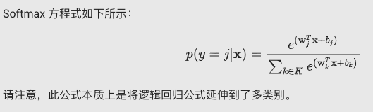
看到这个公式我是一脸懵逼的，看看人家的解释：
https://blog.csdn.net/bitcarmanlee/article/details/82320853

2-2 Softmax 选项

请查看以下 Softmax 变体：

完整 Softmax 是我们一直以来讨论的 Softmax；也就是说，Softmax 针对每个可能的类别计算概率。例如：分别一堆狗照片(首先它确定是只?)的狗品种。
候选采样指 Softmax 针对所有正类别标签计算概率，但仅针对负类别标签的随机样本计算概率。例如，如果我们想要确定某个输入图片(它可能不是只?)是小猎犬还是寻血猎犬图片，则不必针对每个非狗狗样本提供概率。

类别数量较少时，完整 Softmax 代价很小，但随着类别数量的增加，它的代价会变得极其高昂。候选采样可以提高处理具有大量类别的问题的效率。

2-3 一个标签与多个标签

Softmax 假设每个样本只是一个类别的成员。但是，一些样本可以同时是多个类别的成员。对于此类示例：

您不能使用 Softmax。
您必须依赖多个逻辑回归。
例如，假设您的样本是只包含一项内容（一块水果）的图片。Softmax 可以确定该内容是梨、橙子、苹果等的概率。如果您的样本是包含各种各样内容（几碗不同种类的水果）的图片，您必须改用多个逻辑回归。

3 编程练习

在这里插入图片描述

我们的目标是将每个输入图片与正确的数字相对应。我们会创建一个包含几个隐藏层的神经网络，并在顶部放置一个归一化指数层，以选出最合适的类别。

ps:终于有点不一样的栗子了，鸡动

3-1 加载数据集

请注意，此数据是原始 MNIST 训练数据的样本；我们随机选择了 20000 行。
ps：关于MNIST可以先做个简单的了解https://blog.csdn.net/simple_the_best/article/details/75267863
在这里插入图片描述
第一列中包含类别标签，比如5398行的数字是个8。后面其余列中包含特征值，每个像素对应一个特征值，有 28×28=784 个像素值，其中大部分像素值都为零；您也许需要花一分钟时间来确认它们不全部为零。

0-9 这十个数字中的每个可能出现的数字均由唯一的类别标签表示。因此，这是一个具有 10 个类别的多类别分类问题。

3-2 特征和标签

def parse_labels_and_features(dataset):
  """Extracts labels and features.
  
  This is a good place to scale or transform the features if needed.
  
  Args:
    dataset: A Pandas `Dataframe`, containing the label on the first column and
      monochrome pixel values on the remaining columns, in row major order.
  Returns:
    A `tuple` `(labels, features)`:
      labels: A Pandas `Series`.
      features: A Pandas `DataFrame`.
  """
  labels = dataset[0]

  # DataFrame.loc index ranges are inclusive at both ends.
  features = dataset.loc[:,1:784]
  # Scale the data to [0, 1] by dividing out the max value, 255.
  features = features / 255

  return labels, features

知识扩展：
1）dataset.loc[:,1:784] 原型为pandas.DataFrame.loc
打印features，可以知道“,”左边指的是行（所有行），右边是列（1-784列）
比如接下来的：

training_targets, training_examples = parse_labels_and_features(mnist_dataframe[:7500])
training_examples.describe()

从数据集中选取前7500行，最后结果为（7500*784）：
在这里插入图片描述

validation_targets, validation_examples = parse_labels_and_features(mnist_dataframe[7500:10000])
validation_examples.describe()

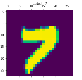
随机打印一个样本及其对应的标签

rand_example = np.random.choice(training_examples.index)
_, ax = plt.subplots()
ax.matshow(training_examples.loc[rand_example].values.reshape(28, 28))
ax.set_title("Label: %i" % training_targets.loc[rand_example])
ax.grid(False)

在这里插入图片描述
知识扩展：

print(training_examples.index)
print(rand_example)
print(training_examples.loc[rand_example])

在这里插入图片描述
1）training_examples是7500*784的dataframe，training_examples.index拿到其所有行的下标
2）np.random.choice 从列表中随机选择一个元素，这里选出了5277
3）training_examples.loc[rand_example] 得到5277行的数据, 后面.values很明显就是拿到1-784列的像素值了。

任务 1：为 MNIST 构建线性模型

首先，我们创建一个基准模型，作为比较对象。LinearClassifier 可提供一组 k* 类一对多分类器，每个类别（共 *k 个）对应一个分类器。

您会发现，除了报告准确率和绘制对数损失函数随时间变化情况的曲线图之外，我们还展示了一个混淆矩阵。混淆矩阵会显示错误分类为其他类别的类别。哪些数字相互之间容易混淆？

另请注意，我们会使用 log_loss 函数跟踪模型的错误。不应将此函数与用于训练的 LinearClassifier 内部损失函数相混淆。

#构建特征列
def construct_feature_columns():
  """Construct the TensorFlow Feature Columns.

  Returns:
    A set of feature columns
  """ 
  
  # There are 784 pixels in each image. 
  return set([tf.feature_column.numeric_column('pixels', shape=784)])

ps：这个特征列的pixels是没有的，因为数据集里面不像前面加利福利亚州的数据都有列名，这里没有，后面构建一个dataframe[‘pixels’]就可以了

在本次练习中，我们会对训练和预测使用单独的输入函数，并将这些函数分别嵌套在 create_training_input_fn() 和 create_predict_input_fn() 中，这样一来，我们就可以调用这些函数，以返回相应的 _input_fn，并将其传递到 .train() 和 .predict() 调用。

def create_training_input_fn(features, labels, batch_size, num_epochs=None, shuffle=True):
  """A custom input_fn for sending MNIST data to the estimator for training.

  Args:
    features: The training features.
    labels: The training labels.
    batch_size: Batch size to use during training.

  Returns:
    A function that returns batches of training features and labels during
    training.
  """
  def _input_fn(num_epochs=None, shuffle=True):
    # Input pipelines are reset with each call to .train(). To ensure model
    # gets a good sampling of data, even when number of steps is small, we 
    # shuffle all the data before creating the Dataset object
    idx = np.random.permutation(features.index)
    raw_features = {"pixels":features.reindex(idx)}
    raw_targets = np.array(labels[idx])
   
    ds = Dataset.from_tensor_slices((raw_features,raw_targets)) # warning: 2GB limit
    ds = ds.batch(batch_size).repeat(num_epochs)
    
    if shuffle:
      ds = ds.shuffle(10000)
    
    # Return the next batch of data.
    feature_batch, label_batch = ds.make_one_shot_iterator().get_next()
    return feature_batch, label_batch

  return _input_fn

def create_predict_input_fn(features, labels, batch_size):
  """A custom input_fn for sending mnist data to the estimator for predictions.

  Args:
    features: The features to base predictions on.
    labels: The labels of the prediction examples.

  Returns:
    A function that returns features and labels for predictions.
  """
  def _input_fn():
    raw_features = {"pixels": features.values}
    raw_targets = np.array(labels)
    
    ds = Dataset.from_tensor_slices((raw_features, raw_targets)) # warning: 2GB limit
    ds = ds.batch(batch_size)
    
        
    # Return the next batch of data.
    feature_batch, label_batch = ds.make_one_shot_iterator().get_next()
    return feature_batch, label_batch

  return _input_fn

ps:这次将输入函数分成了训练输入函数和预测输入函数。可以看到下面一个create_predict_input_fn的代码是比较清晰的，
在这里插入图片描述
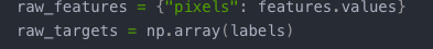
构建Dataset.from_tensor_slices所需要的参数，前面了解过，特征项需要是个dict，里面的value是个Series, 标签项需要Series，后面再分片。

至于上面的那个create_training_input_fn，里面有这样的一步
在这里插入图片描述
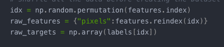
np.random.permutation将features的顺序随机化，然后对应的特征和标签同步处理，就是随机化的过程

def train_linear_classification_model(
    learning_rate,
    steps,
    batch_size,
    training_examples,
    training_targets,
    validation_examples,
    validation_targets):
  """Trains a linear classification model for the MNIST digits dataset.
  
  In addition to training, this function also prints training progress information,
  a plot of the training and validation loss over time, and a confusion
  matrix.
  
  Args:
    learning_rate: An `int`, the learning rate to use.
    steps: A non-zero `int`, the total number of training steps. A training step
      consists of a forward and backward pass using a single batch.
    batch_size: A non-zero `int`, the batch size.
    training_examples: A `DataFrame` containing the training features.
    training_targets: A `DataFrame` containing the training labels.
    validation_examples: A `DataFrame` containing the validation features.
    validation_targets: A `DataFrame` containing the validation labels.
      
  Returns:
    The trained `LinearClassifier` object.
  """

  periods = 10

  steps_per_period = steps / periods  
  # Create the input functions.
  predict_training_input_fn = create_predict_input_fn(
    training_examples, training_targets, batch_size)
  predict_validation_input_fn = create_predict_input_fn(
    validation_examples, validation_targets, batch_size)
  training_input_fn = create_training_input_fn(
    training_examples, training_targets, batch_size)
  
  # Create a LinearClassifier object.
  my_optimizer = tf.train.AdagradOptimizer(learning_rate=learning_rate)
  my_optimizer = tf.contrib.estimator.clip_gradients_by_norm(my_optimizer, 5.0)
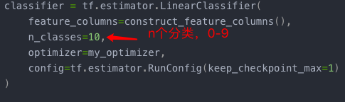
  classifier = tf.estimator.LinearClassifier(
      feature_columns=construct_feature_columns(),
      n_classes=10,
      optimizer=my_optimizer,
      config=tf.estimator.RunConfig(keep_checkpoint_max=1)
  )

  # Train the model, but do so inside a loop so that we can periodically assess
  # loss metrics.
  print("Training model...")
  print("LogLoss error (on validation data):")
  training_errors = []
  validation_errors = []
  for period in range (0, periods):
    # Train the model, starting from the prior state.
    classifier.train(
        input_fn=training_input_fn,
        steps=steps_per_period
    )
  
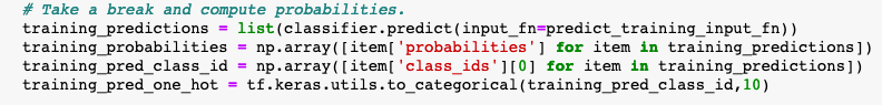
    # Take a break and compute probabilities.
    training_predictions = list(classifier.predict(input_fn=predict_training_input_fn))
    training_probabilities = np.array([item['probabilities'] for item in training_predictions])
    training_pred_class_id = np.array([item['class_ids'][0] for item in training_predictions])
    training_pred_one_hot = tf.keras.utils.to_categorical(training_pred_class_id,10)
    
   
        
    validation_predictions = list(classifier.predict(input_fn=predict_validation_input_fn))
    validation_probabilities = np.array([item['probabilities'] for item in validation_predictions])    
    validation_pred_class_id = np.array([item['class_ids'][0] for item in validation_predictions])
    validation_pred_one_hot = tf.keras.utils.to_categorical(validation_pred_class_id,10)    
    
    # Compute training and validation errors.
    training_log_loss = metrics.log_loss(training_targets, training_pred_one_hot)
    validation_log_loss = metrics.log_loss(validation_targets, validation_pred_one_hot)
    # Occasionally print the current loss.
    print("  period %02d : %0.2f" % (period, validation_log_loss))
    # Add the loss metrics from this period to our list.
    training_errors.append(training_log_loss)
    validation_errors.append(validation_log_loss)
  print("Model training finished.")
  # Remove event files to save disk space.
  print('classifier.model_dir: ',classifier.model_dir)
  _ = map(os.remove, glob.glob(os.path.join(classifier.model_dir, 'events.out.tfevents*')))
  
  # Calculate final predictions (not probabilities, as above).
  final_predictions = classifier.predict(input_fn=predict_validation_input_fn)
  final_predictions = np.array([item['class_ids'][0] for item in final_predictions])
  
  
  accuracy = metrics.accuracy_score(validation_targets, final_predictions)
  print("Final accuracy (on validation data): %0.2f" % accuracy)

  # Output a graph of loss metrics over periods.
  plt.ylabel("LogLoss")
  plt.xlabel("Periods")
  plt.title("LogLoss vs. Periods")
  plt.plot(training_errors, label="training")
  plt.plot(validation_errors, label="validation")
  plt.legend()
  plt.show()
  
  # Output a plot of the confusion matrix.
  cm = metrics.confusion_matrix(validation_targets, final_predictions)
  # Normalize the confusion matrix by row (i.e by the number of samples
  # in each class).
  cm_normalized = cm.astype("float") / cm.sum(axis=1)[:, np.newaxis]
  ax = sns.heatmap(cm_normalized, cmap="bone_r")
  ax.set_aspect(1)
  plt.title("Confusion matrix")
  plt.ylabel("True label")
  plt.xlabel("Predicted label")
  plt.show()

  return classifier

知识扩展：

看看这段在干啥子

打印一下

前面了解过，item[‘probabilities’]可以从预测结果中拿到预测的值,这是个矩阵啊，打印一下：

print('len_training_probabilities',len(training_probabilities),'len_element',len(training_probabilities[0]))

在这里插入图片描述
这是个7500x10的矩阵,7500我知道是训练集的长度，10是什么？前面任务1有句描述‘LinearClassifier 可提供一组 k* 类一对多分类器，每个类别（共 *k 个）对应一个分类器。’, 我严重怀疑这里是0-9的概率，合值应该是1，随便找个样本打印一下：
print(‘sum’,sum(training_probabilities[1]))
在这里插入图片描述
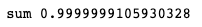
差不多哈，那这个10在哪指定的呢？前面定义LinearClassifier的时候

好既然这样，接下来就好说了，training_pred_class_id则代表这7500个样本被分到的类别中，也就相当于预测的数字。

最后，这个training_pred_one_hot = tf.keras.utils.to_categorical(training_pred_class_id,10) 又是在干嘛?，又打印了个矩阵，我们来看看它的size。

print('training_pred_one_hot',len(training_pred_one_hot),'len_el',len(training_pred_one_hot[1]))

在这里插入图片描述
又是个7500*10,看看官方的解释

将一个整型的数组转换为0，1值的矩阵

2）关于log_loss，好像是说，log(0)会变成无穷大，所以sklearn提供了转换成一个极小值，有兴趣的可以研究下
https://blog.csdn.net/ybdesire/article/details/73695163

3）最后一段：
在这里插入图片描述
这是任务1说的混淆矩阵，混淆矩阵会显示错误分类为其他类别的类别。
长这样的

其中对角线上的，都是预测正确的，其他位置是预测错误的。详解可以看看这个：
https://blog.csdn.net/m0_38061927/article/details/77198990

可以看出其他位置占比比较小，对角线上颜色较深，占比大，这个预测还比较准

执行训练

classifier = train_linear_classification_model(
             learning_rate=0.02,
             steps=100,
             batch_size=10,
             training_examples=training_examples,
             training_targets=training_targets,
             validation_examples=validation_examples,
             validation_targets=validation_targets)

在这里插入图片描述
可以看到准确率0.84没有达到0.9，需要对超参数进行调整。

classifier = train_linear_classification_model(
             learning_rate=0.024,
             steps=1000,
             batch_size=50,
             training_examples=training_examples,
             training_targets=training_targets,
             validation_examples=validation_examples,
             validation_targets=validation_targets)

在这里插入图片描述
好像收敛的不是特别好，但是站上了0.91

任务2：使用神经网络替换线性分类器

使用 DNNClassifier 替换上面的 LinearClassifier，并查找可实现 0.95 或更高准确率的参数组合。

您可能希望尝试 Dropout 等其他正则化方法。这些额外的正则化方法已记录在 DNNClassifier 类的注释中。

除了神经网络专用配置（例如隐藏单元的超参数）之外，以下代码与原始的 LinearClassifer 训练代码几乎完全相同。

def train_nn_classification_model(
    learning_rate,
    steps,
    batch_size,
    hidden_units,
    training_examples,
    training_targets,
    validation_examples,
    validation_targets):
  """Trains a neural network classification model for the MNIST digits dataset.
  
  In addition to training, this function also prints training progress information,
  a plot of the training and validation loss over time, as well as a confusion
  matrix.
  
  Args:
    learning_rate: An `int`, the learning rate to use.
    steps: A non-zero `int`, the total number of training steps. A training step
      consists of a forward and backward pass using a single batch.
    batch_size: A non-zero `int`, the batch size.
    hidden_units: A `list` of int values, specifying the number of neurons in each layer.
    training_examples: A `DataFrame` containing the training features.
    training_targets: A `DataFrame` containing the training labels.
    validation_examples: A `DataFrame` containing the validation features.
    validation_targets: A `DataFrame` containing the validation labels.
      
  Returns:
    The trained `DNNClassifier` object.
  """

  periods = 10
  # Caution: input pipelines are reset with each call to train. 
  # If the number of steps is small, your model may never see most of the data.  
  # So with multiple `.train` calls like this you may want to control the length 
  # of training with num_epochs passed to the input_fn. Or, you can do a really-big shuffle, 
  # or since it's in-memory data, shuffle all the data in the `input_fn`.
  steps_per_period = steps / periods  
  # Create the input functions.
  predict_training_input_fn = create_predict_input_fn(
    training_examples, training_targets, batch_size)
  predict_validation_input_fn = create_predict_input_fn(
    validation_examples, validation_targets, batch_size)
  training_input_fn = create_training_input_fn(
    training_examples, training_targets, batch_size)
  
  # Create the input functions.
  predict_training_input_fn = create_predict_input_fn(
    training_examples, training_targets, batch_size)
  predict_validation_input_fn = create_predict_input_fn(
    validation_examples, validation_targets, batch_size)
  training_input_fn = create_training_input_fn(
    training_examples, training_targets, batch_size)
  
  # Create feature columns.
  feature_columns = [tf.feature_column.numeric_column('pixels', shape=784)]

  # Create a DNNClassifier object.
  my_optimizer = tf.train.AdagradOptimizer(learning_rate=learning_rate)
  my_optimizer = tf.contrib.estimator.clip_gradients_by_norm(my_optimizer, 5.0)
  classifier = tf.estimator.DNNClassifier(
      feature_columns=feature_columns,
      n_classes=10,
      hidden_units=hidden_units,
      optimizer=my_optimizer,
      config=tf.contrib.learn.RunConfig(keep_checkpoint_max=1)
  )

  # Train the model, but do so inside a loop so that we can periodically assess
  # loss metrics.
  print("Training model...")
  print("LogLoss error (on validation data):")
  training_errors = []
  validation_errors = []
  for period in range (0, periods):
    # Train the model, starting from the prior state.
    classifier.train(
        input_fn=training_input_fn,
        steps=steps_per_period
    )
  
    # Take a break and compute probabilities.
    training_predictions = list(classifier.predict(input_fn=predict_training_input_fn))
    training_probabilities = np.array([item['probabilities'] for item in training_predictions])
    training_pred_class_id = np.array([item['class_ids'][0] for item in training_predictions])
    training_pred_one_hot = tf.keras.utils.to_categorical(training_pred_class_id,10)
        
    validation_predictions = list(classifier.predict(input_fn=predict_validation_input_fn))
    validation_probabilities = np.array([item['probabilities'] for item in validation_predictions])    
    validation_pred_class_id = np.array([item['class_ids'][0] for item in validation_predictions])
    validation_pred_one_hot = tf.keras.utils.to_categorical(validation_pred_class_id,10)    
    
    # Compute training and validation errors.
    training_log_loss = metrics.log_loss(training_targets, training_pred_one_hot)
    validation_log_loss = metrics.log_loss(validation_targets, validation_pred_one_hot)
    # Occasionally print the current loss.
    print("  period %02d : %0.2f" % (period, validation_log_loss))
    # Add the loss metrics from this period to our list.
    training_errors.append(training_log_loss)
    validation_errors.append(validation_log_loss)
  print("Model training finished.")
  # Remove event files to save disk space.
  _ = map(os.remove, glob.glob(os.path.join(classifier.model_dir, 'events.out.tfevents*')))
  
  # Calculate final predictions (not probabilities, as above).
  final_predictions = classifier.predict(input_fn=predict_validation_input_fn)
  final_predictions = np.array([item['class_ids'][0] for item in final_predictions])
  
  
  accuracy = metrics.accuracy_score(validation_targets, final_predictions)
  print("Final accuracy (on validation data): %0.2f" % accuracy)

  # Output a graph of loss metrics over periods.
  plt.ylabel("LogLoss")
  plt.xlabel("Periods")
  plt.title("LogLoss vs. Periods")
  plt.plot(training_errors, label="training")
  plt.plot(validation_errors, label="validation")
  plt.legend()
  plt.show()
  
  # Output a plot of the confusion matrix.
  cm = metrics.confusion_matrix(validation_targets, final_predictions)
  # Normalize the confusion matrix by row (i.e by the number of samples
  # in each class).
  cm_normalized = cm.astype("float") / cm.sum(axis=1)[:, np.newaxis]
  ax = sns.heatmap(cm_normalized, cmap="bone_r")
  ax.set_aspect(1)
  plt.title("Confusion matrix")
  plt.ylabel("True label")
  plt.xlabel("Predicted label")
  plt.show()

  return classifier

目标是0.95以上，调节下训练参数

classifier = train_nn_classification_model(
    learning_rate=0.05,
    steps=1000,
    batch_size=30,
    hidden_units=[20, 15,10],
    training_examples=training_examples,
    training_targets=training_targets,
    validation_examples=validation_examples,
    validation_targets=validation_targets)

在这里插入图片描述
发现还是不太够，目测还要加节点。为了节省时间我还是不慢慢试了，以下是官方答案：(100x100啊，?)

classifier = train_nn_classification_model(
    learning_rate=0.05,
    steps=1000,
    batch_size=30,
    hidden_units=[100, 100],
    training_examples=training_examples,
    training_targets=training_targets,
    validation_examples=validation_examples,
    validation_targets=validation_targets)

在这里插入图片描述

在这里插入图片描述
ps：像这种一片黑的就对了

后面是测试集测试：

mnist_test_dataframe = pd.read_csv(
  "https://download.mlcc.google.cn/mledu-datasets/mnist_test.csv",
  sep=",",
  header=None)

test_targets, test_examples = parse_labels_and_features(mnist_test_dataframe)
test_examples.describe()

predict_test_input_fn = create_predict_input_fn(
    test_examples, test_targets, batch_size=100)

test_predictions = classifier.predict(input_fn=predict_test_input_fn)
test_predictions = np.array([item['class_ids'][0] for item in test_predictions])
  
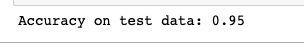
accuracy = metrics.accuracy_score(test_targets, test_predictions)
print("Accuracy on test data: %0.2f" % accuracy)

这里也不说了，仿造上面的代码就行
在这里插入图片描述

任务 3：可视化第一个隐藏层的权重。

我们来花几分钟时间看看模型的 weights_ 属性，以深入探索我们的神经网络，并了解它学到了哪些规律。

模型的输入层有 784 个权重，对应于 28×28 像素输入图片。第一个隐藏层将有 784×N 个权重，其中 N 指的是该层中的节点数。我们可以将这些权重重新变回 28×28 像素的图片，具体方法是将 N 个 1×784 权重数组变形为 N 个 28×28 大小数组。

1）运行以下单元格，绘制权重曲线图。请注意，此单元格要求名为 “classifier” 的 DNNClassifier 已经过训练。

print(classifier.get_variable_names())

weights0 = classifier.get_variable_value("dnn/hiddenlayer_0/kernel")

print("weights0 shape:", weights0.shape)

num_nodes = weights0.shape[1]
num_rows = int(math.ceil(num_nodes / 10.0))
fig, axes = plt.subplots(num_rows, 10, figsize=(20, 2 * num_rows))
for coef, ax in zip(weights0.T, axes.ravel()):
    # Weights in coef is reshaped from 1x784 to 28x28.
    ax.matshow(coef.reshape(28, 28), cmap=plt.cm.pink)
    ax.set_xticks(())
    ax.set_yticks(())

plt.show()

在这里插入图片描述

神经网络的第一个隐藏层应该会对一些级别特别低的特征进行建模，因此可视化权重可能只显示一些模糊的区域，也可能只显示数字的某几个部分。此外，您可能还会看到一些基本上是噪点（这些噪点要么不收敛，要么被更高的层忽略）的神经元。

在迭代不同的次数后停止训练并查看效果，可能会发现有趣的结果。

分别用 10、100 和 1000 步训练分类器。然后重新运行此可视化。

您看到不同级别的收敛之间有哪些直观上的差异？

ps：刚才已经跑了1000步训练的分类器，由于设置的是[100,100]，两层，每层100个节点。第一层的图看起来确实很模糊。

2）根据提示，再做100步训练,batch_size当然跟着减小一点

classifier = train_nn_classification_model(
    learning_rate=0.05,
    steps=100,
    batch_size=10,
    hidden_units=[100, 100],
    training_examples=training_examples,
    training_targets=training_targets,
    validation_examples=validation_examples,
    validation_targets=validation_targets)

在不断跑的时候发现报错了。忘了截图了，最后的原因是我的磁盘空间居然满了，在跑的时候不断有这个提示：
在这里插入图片描述
后来发现这个模型会产生输出文件，很大很大，一次一个多G?。

细心的同志会发现里面有个清理的代码,我把位置顺便打印了出来：

# Remove event files to save disk space.
  _ = map(os.remove, glob.glob(os.path.join(classifier.model_dir, 'events.out.tfevents*')))
  print("path: ",os.path.join(classifier.model_dir, 'events.out.tfevents*'))

发现是存在这里的path: /var/folders/4s/q7gxlvx1493czfrmqd1knhqc0000gn/T/tmp5tyxib3x/events.out.tfevents*

进去果然发现了大量没有删除的temp临时文件。不要乱删哦，有其他软件的文件也在T里面。把这个tmpxxx都删掉就干净了。少了近80G，我去，最近跑了不少模型啊。

在这里插入图片描述

Final accuracy (on validation data): 0.82
跟1000步的比貌似，这种发散的节点多了些

收敛的节点少了

3）最后在做10步的

classifier = train_nn_classification_model(
    learning_rate=0.05,
    steps=10,
    batch_size=1,
    hidden_units=[100, 100],
    training_examples=training_examples,
    training_targets=training_targets,
    validation_examples=validation_examples,
    validation_targets=validation_targets)

Final accuracy (on validation data): 0.19

ps:果然准确率低的令人发指，应该也是大片的发散，收敛的少
在这里插入图片描述

ps：好吧，看来还高估了，基本都是发散的，那0.19的正确率是靠蒙的吧?

狂奔的CD

关注

0
点赞
踩
1

收藏

觉得还不错? 一键收藏
0
评论
人工智能小白日记之16 ML学习篇之12多类别神经网络 Multi-Class Neural Networks

人工智能小白日记之16 ML学习篇之12多类别神经网络 Multi-Class Neural Networks前言课程内容1 一对多2 softmax2-1 Softmax方程式2-2 Softmax 选项2-3 一个标签与多个标签前言前面已经了解了二元分类问题，比如这张图片是不是小狗
复制链接

扫一扫