吴恩达深度学习编程作业（2-1）- Initialization & Regularization & Gradient Checking

最新推荐文章于 2024-07-13 11:34:52 发布

大树先生的博客

最新推荐文章于 2024-07-13 11:34:52 发布

阅读量1.5w

点赞数 18

分类专栏：吴恩达深度学习编程作业文章标签：深度学习改善深层神经网络超参数正则化梯度检验

本文链接：https://blog.csdn.net/koala_tree/article/details/78137306

版权

吴恩达Coursera课程 DeepLearning.ai 编程作业系列，本文为《改善深层神经网络：超参数调试、正则化以及优化》部分的第四周“深度学习的实践方面”的课程作业，同时增加了一些辅助的测试函数。

另外，本节课程笔记在此：《吴恩达Coursera深度学习课程 DeepLearning.ai 提炼笔记（2-1）– 深度学习的实践方面》，如有任何建议和问题，欢迎留言。

You can get the support code and datasets from here for all the following parts.

Part 1：Initialization

A well chosen initialization can:
- Speed up the convergence of gradient descent
- Increase the odds of gradient descent converging to a lower training (and generalization) error

To get started, run the following cell to load the packages and the planar dataset you will try to classify.

import numpy as np
import matplotlib.pyplot as plt
import sklearn
import sklearn.datasets
from init_utils import sigmoid, relu, compute_loss, forward_propagation, backward_propagation
from init_utils import update_parameters, predict, load_dataset, plot_decision_boundary, predict_dec

%matplotlib inline
plt.rcParams['figure.figsize'] = (7.0, 4.0) # set default size of plots
plt.rcParams['image.interpolation'] = 'nearest'
plt.rcParams['image.cmap'] = 'gray'

# load image dataset: blue/red dots in circles
train_X, train_Y, test_X, test_Y = load_dataset()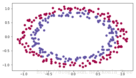

There are some import function：

def sigmoid(x):
    """
    Compute the sigmoid of x

    Arguments:
    x -- A scalar or numpy array of any size.

    Return:
    s -- sigmoid(x)
    """
    s = 1/(1+np.exp(-x))
    return s


def relu(x):
    """
    Compute the relu of x

    Arguments:
    x -- A scalar or numpy array of any size.

    Return:
    s -- relu(x)
    """
    s = np.maximum(0,x)

    return s


def compute_loss(a3, Y):

    """
    Implement the loss function

    Arguments:
    a3 -- post-activation, output of forward propagation
    Y -- "true" labels vector, same shape as a3

    Returns:
    loss - value of the loss function
    """

    m = Y.shape[1]
    logprobs = np.multiply(-np.log(a3),Y) + np.multiply(-np.log(1 - a3), 1 - Y)
    loss = 1./m * np.nansum(logprobs)

    return loss

def forward_propagation(X, parameters):
    """
    Implements the forward propagation (and computes the loss) presented in Figure 2.

    Arguments:
    X -- input dataset, of shape (input size, number of examples)
    Y -- true "label" vector (containing 0 if cat, 1 if non-cat)
    parameters -- python dictionary containing your parameters "W1", "b1", "W2", "b2", "W3", "b3":
                    W1 -- weight matrix of shape ()
                    b1 -- bias vector of shape ()
                    W2 -- weight matrix of shape ()
                    b2 -- bias vector of shape ()
                    W3 -- weight matrix of shape ()
                    b3 -- bias vector of shape ()

    Returns:
    loss -- the loss function (vanilla logistic loss)
    """

    # retrieve parameters
    W1 = parameters["W1"]
    b1 = parameters["b1"]
    W2 = parameters["W2"]
    b2 = parameters["b2"]
    W3 = parameters["W3"]
    b3 = parameters["b3"]

    # LINEAR -> RELU -> LINEAR -> RELU -> LINEAR -> SIGMOID
    z1 = np.dot(W1, X) + b1
    a1 = relu(z1)
    z2 = np.dot(W2, a1) + b2
    a2 = relu(z2)
    z3 = np.dot(W3, a2) + b3
    a3 = sigmoid(z3)

    cache = (z1, a1, W1, b1, z2, a2, W2, b2, z3, a3, W3, b3)

    return a3, cache


def backward_propagation(X, Y, cache):
    """
    Implement the backward propagation presented in figure 2.

    Arguments:
    X -- input dataset, of shape (input size, number of examples)
    Y -- true "label" vector (containing 0 if cat, 1 if non-cat)
    cache -- cache output from forward_propagation()

    Returns:
    gradients -- A dictionary with the gradients with respect to each parameter, activation and pre-activation variables
    """
    m = X.shape[1]
    (z1, a1, W1, b1, z2, a2, W2, b2, z3, a3, W3, b3) = cache

    dz3 = 1./m * (a3 - Y)
    dW3 = np.dot(dz3, a2.T)
    db3 = np.sum(dz3, axis=1, keepdims = True)

    da2 = np.dot(W3.T, dz3)
    dz2 = np.multiply(da2, np.int64(a2 > 0))
    dW2 = np.dot(dz2, a1.T)
    db2 = np.sum(dz2, axis=1, keepdims = True)

    da1 = np.dot(W2.T, dz2)
    dz1 = np.multiply(da1, np.int64(a1 > 0))
    dW1 = np.dot(dz1, X.T)
    db1 = np.sum(dz1, axis=1, keepdims = True)

    gradients = {
  "dz3": dz3, "dW3": dW3, "db3": db3,
                 "da2": da2, "dz2": dz2, "dW2": dW2, "db2": db2,
                 "da1": da1, "dz1": dz1, "dW1": dW1, "db1": db1}

    return gradients


def update_parameters(parameters, grads, learning_rate):
    """
    Update parameters using gradient descent

    Arguments:
    parameters -- python dictionary containing your parameters 
    grads -- python dictionary containing your gradients, output of n_model_backward

    Returns:
    parameters -- python dictionary containing your updated parameters 
                  parameters['W' + str(i)] = ... 
                  parameters['b' + str(i)] = ...
    """

    L = len(parameters) // 2 # number of layers in the neural networks

    # Update rule for each parameter
    for k in range(L):
        parameters["W" + str(k+1)] = parameters["W" + str(k+1)] - learning_rate * grads["dW" + str(k+1)]
        parameters["b" + str(k+1)] = parameters["b" + str(k+1)] - learning_rate * grads["db" + str(k+1)]

    return parameters


def predict(X, y, parameters):
    """
    This function is used to predict the results of a  n-layer neural network.

    Arguments:
    X -- data set of examples you would like to label
    parameters -- parameters of the trained model

    Returns:
    p -- predictions for the given dataset X
    """

    m = X.shape[1]
    p = np.zeros((1,m), dtype = np.int)

    # Forward propagation
    a3, caches = forward_propagation(X, parameters)

    # convert probas to 0/1 predictions
    for i in range(0, a3.shape[1]):
        if a3[0,i] > 0.5:
            p[0,i] = 1
        else:
            p[0,i] = 0

    # print results
    print("Accuracy: "  + str(np.mean((p[0,:] == y[0,:]))))

    return p


def load_dataset():
    np.random.seed(1)
    train_X, train_Y = sklearn.datasets.make_circles(n_samples=300, noise=.05)
    np.random.seed(2)
    test_X, test_Y = sklearn.datasets.make_circles(n_samples=100, noise=.05)
    # Visualize the data
    plt.scatter(train_X[:, 0], train_X[:, 1], c=train_Y, s=40, cmap=plt.cm.Spectral);
    train_X = train_X.T
    train_Y = train_Y.reshape((1, train_Y.shape[0]))
    test_X = test_X.T
    test_Y = test_Y.reshape((1, test_Y.shape[0]))
    return train_X, train_Y, test_X, test_Y


def plot_decision_boundary(model, X, y):
    # Set min and max values and give it some padding
    x_min, x_max = X[0, :].min() - 1, X[0, :].max() + 1
    y_min, y_max = X[1, :].min() - 1, X[1, :].max() + 1
    h = 0.01
    # Generate a grid of points with distance h between them
    xx, yy = np.meshgrid(np.arange(x_min, x_max, h), np.arange(y_min, y_max, h))
    # Predict the function value for the whole grid
    Z = model(np.c_[xx.ravel(), yy.ravel()])
    Z = Z.reshape(xx.shape)
    # Plot the contour and training examples
    plt.contourf(xx, yy, Z, cmap=plt.cm.Spectral)
    plt.ylabel('x2')
    plt.xlabel('x1')
    plt.scatter(X[0, :], X[1, :], c=y, cmap=plt.cm.Spectral)
    plt.show()


def predict_dec(parameters, X):
    """
    Used for plotting decision boundary.

    Arguments:
    parameters -- python dictionary containing your parameters 
    X -- input data of size (m, K)

    Returns
    predictions -- vector of predictions of our model (red: 0 / blue: 1)
    """

    # Predict using forward propagation and a classification threshold of 0.5
    a3, cache = forward_propagation(X, parameters)
    predictions = (a3>0.5)
    return predictions

You would like a classifier to separate the blue dots from the red dots.

1 - Neural Network model

You will use a 3-layer neural network (already implemented for you). Here are the initialization methods you will experiment with:
- Zeros initialization – setting initialization = "zeros" in the input argument.
- Random initialization – setting initialization = "random" in the input argument. This initializes the weights to large random values.
- He initialization – setting initialization = "he" in the input argument. This initializes the weights to random values scaled according to a paper by He et al., 2015.

Instructions: Please quickly read over the code below, and run it. In the next part you will implement the three initialization methods that this model() calls.

def model(X, Y, learning_rate = 0.01, num_iterations = 15000, print_cost = True, initialization = "he"):
    """
    Implements a three-layer neural network: LINEAR->RELU->LINEAR->RELU->LINEAR->SIGMOID.

    Arguments:
    X -- input data, of shape (2, number of examples)
    Y -- true "label" vector (containing 0 for red dots; 1 for blue dots), of shape (1, number of examples)
    learning_rate -- learning rate for gradient descent 
    num_iterations -- number of iterations to run gradient descent
    print_cost -- if True, print the cost every 1000 iterations
    initialization -- flag to choose which initialization to use ("zeros","random" or "he")

    Returns:
    parameters -- parameters learnt by the model
    """

    grads = {}
    costs = [] # to keep track of the loss
    m = X.shape[1] # number of examples
    layers_dims = [X.shape[0], 10, 5, 1]

    # Initialize parameters dictionary.
    if initialization == "zeros":
        parameters = initialize_parameters_zeros(layers_dims)
    elif initialization == "random":
        parameters = initialize_parameters_random(layers_dims)
    elif initialization == "he":
        parameters = initialize_parameters_he(layers_dims)

    # Loop (gradient descent)

    for i in range(0, num_iterations):

        # Forward propagation: LINEAR -> RELU -> LINEAR -> RELU -> LINEAR -> SIGMOID.
        a3, cache = forward_propagation(X, parameters)

        # Loss
        cost = compute_loss(a3, Y)

        # Backward propagation.
        grads = backward_propagation(X, Y, cache)

        # Update parameters.
        parameters = update_parameters(parameters, grads, learning_rate)

        # Print the loss every 1000 iterations
        if print_cost and i % 1000 == 0:
            print("Cost after iteration {}: {}".format(i, cost))
            costs.append(cost)

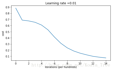
    # plot the loss
    plt.plot(costs)
    plt.ylabel('cost')
    plt.xlabel('iterations (per hundreds)')
    plt.title("Learning rate =" + str(learning_rate))
    plt.show()

    return parameters

2 - Zero initialization

There are two types of parameters to initialize in a neural network:
- the weight matrices $(W^{[1]}, W^{[2]}, W^{[3]}, ..., W^{[L-1]}, W^{[L]})$
- the bias vectors $(b^{[1]}, b^{[2]}, b^{[3]}, ..., b^{[L-1]}, b^{[L]})$

Exercise: Implement the following function to initialize all parameters to zeros. You’ll see later that this does not work well since it fails to “break symmetry”, but lets try it anyway and see what happens. Use np.zeros((..,..)) with the correct shapes.

# GRADED FUNCTION: initialize_parameters_zeros 

def initialize_parameters_zeros(layers_dims):
    """
    Arguments:
    layer_dims -- python array (list) containing the size of each layer.

    Returns:
    parameters -- python dictionary containing your parameters "W1", "b1", ..., "WL", "bL":
                    W1 -- weight matrix of shape (layers_dims[1], layers_dims[0])
                    b1 -- bias vector of shape (layers_dims[1], 1)
                    ...
                    WL -- weight matrix of shape (layers_dims[L], layers_dims[L-1])
                    bL -- bias vector of shape (layers_dims[L], 1)
    """

    parameters = {}
    L = len(layers_dims)            # number of layers in the network

    for l in range(1, L):
        ### START CODE HERE ### (≈ 2 lines of code)
        parameters['W' + str(l)] = np.zeros((layers_dims[l],layers_dims[l-1]))
        parameters['b' + str(l)] = np.zeros((layers_dims[l],1))
        ### END CODE HERE ###
    return parameters

parameters = initialize_parameters_zeros([3,2,1])
print("W1 = " + str(parameters["W1"]))
print("b1 = " + str(parameters["b1"]))
print("W2 = " + str(parameters["W2"]))
print("b2 = " + str(parameters["b2"]))

W1 = [[ 0.  0.  0.]
 [ 0.  0.  0.]]
b1 = [[ 0.]
 [ 0.]]
W2 = [[ 0.  0.]]
b2 = [[ 0.]]

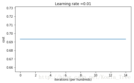
Run the following code to train your model on 15,000 iterations using zeros initialization.

parameters = model(train_X, train_Y, initialization = "zeros")
print ("On the train set:")
predictions_train = predict(train_X, train_Y, parameters)
print ("On the test set:")
predictions_test = predict(test_X, test_Y, parameters)

Cost after iteration 0: 0.6931471805599453
Cost after iteration 1000: 0.6931471805599453
Cost after iteration 2000: 0.6931471805599453
Cost after iteration 3000: 0.6931471805599453
Cost after iteration 4000: 0.6931471805599453
Cost after iteration 5000: 0.6931471805599453
Cost after iteration 6000: 0.6931471805599453
Cost after iteration 7000: 0.6931471805599453
Cost after iteration 8000: 0.6931471805599453
Cost after iteration 9000: 0.6931471805599453
Cost after iteration 10000: 0.6931471805599455
Cost after iteration 11000: 0.6931471805599453
Cost after iteration 12000: 0.6931471805599453
Cost after iteration 13000: 0.6931471805599453
Cost after iteration 14000: 0.6931471805599453

On the train set:
Accuracy: 0.5
On the test set:
Accuracy: 0.5

The performance is really bad, and the cost does not really decrease, and the algorithm performs no better than random guessing. Why? Lets look at the details of the predictions and the decision boundary:

print ("predictions_train = " + str(predictions_train))
print ("predictions_test = " + str(predictions_test))

predictions_train = [[0 0 0 0 0 0 0 0 0 0 0 0 0 0 0 0 0 0 0 0 0 0 0 0 0 0 0 0 0 0 0 0 0 0 0 0 0
  0 0 0 0 0 0 0 0 0 0 0 0 0 0 0 0 0 0 0 0 0 0 0 0 0 0 0 0 0 0 0 0 0 0 0 0 0
  0 0 0 0 0 0 0 0 0 0 0 0 0 0 0 0 0 0 0 0 0 0 0 0 0 0 0 0 0 0 0 0 0 0 0 0 0
  0 0 0 0 0 0 0 0 0 0 0 0 0 0 0 0 0 0 0 0 0 0 0 0 0 0 0 0 0 0 0 0 0 0 0 0 0
  0 0 0 0 0 0 0 0 0 0 0 0 0 0 0 0 0 0 0 0 0 0 0 0 0 0 0 0 0 0 0 0 0 0 0 0 0
  0 0 0 0 0 0 0 0 0 0 0 0 0 0 0 0 0 0 0 0 0 0 0 0 0 0 0 0 0 0 0 0 0 0 0 0 0
  0 0 0 0 0 0 0 0 0 0 0 0 0 0 0 0 0 0 0 0 0 0 0 0 0 0 0 0 0 0 0 0 0 0 0 0 0
  0 0 0 0 0 0 0 0 0 0 0 0 0 0 0 0 0 0 0 0 0 0 0 0 0 0 0 0 0 0 0 0 0 0 0 0 0
  0 0 0 0]]
predictions_test = [[0 0 0 0 0 0 0 0 0 0 0 0 0 0 0 0 0 0 0 0 0 0 0 0 0 0 0 0 0 0 0 0 0 0 0 0 0
  0 0 0 0 0 0 0 0 0 0 0 0 0 0 0 0 0 0 0 0 0 0 0 0 0 0 0 0 0 0 0 0 0 0 0 0 0
  0 0 0 0 0 0 0 0 0 0 0 0 0 0 0 0 0 0 0 0 0 0 0 0 0 0]]

plt.title("Model with Zeros initialization")
axes = plt.gca()
axes.set_xlim([-1.5,1.5])
axes.set_ylim([-1.5,1.5])
plot_decision_boundary(lambda x: predict_dec(parameters, x.T), train_X, train_Y)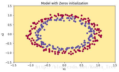

The model is predicting 0 for every example.

In general, initializing all the weights to zero results in the network failing to break symmetry. This means that every neuron in each layer will learn the same thing, and you might as well be training a neural network with $n^{[l]}=1$ for every layer, and the network is no more powerful than a linear classifier such as logistic regression.

What you should remember:
- The weights $W^{[l]}$ should be initialized randomly to break symmetry.
- It is however okay to initialize the biases $b^{[l]}$ to zeros. Symmetry is still broken so long as $W^{[l]}$ is initialized randomly.

3 - Random initialization

To break symmetry, lets intialize the weights randomly. Following random initialization, each neuron can then proceed to learn a different function of its inputs. In this exercise, you will see what happens if the weights are intialized randomly, but to very large values.

Exercise: Implement the following function to initialize your weights to large random values (scaled by *10) and your biases to zeros. Use np.random.randn(..,..) * 10 for weights and np.zeros((.., ..)) for biases. We are using a fixed np.random.seed(..) to make sure your “random” weights match ours, so don’t worry if running several times your code gives you always the same initial values for the parameters.

# GRADED FUNCTION: initialize_parameters_random

def initialize_parameters_random(layers_dims):
    """
    Arguments:
    layer_dims -- python array (list) containing the size of each layer.

    Returns:
    parameters -- python dictionary containing your parameters "W1", "b1", ..., "WL", "bL":
                    W1 -- weight matrix of shape (layers_dims[1], layers_dims[0])
                    b1 -- bias vector of shape (layers_dims[1], 1)
                    ...
                    WL -- weight matrix of shape (layers_dims[L], layers_dims[L-1])
                    bL -- bias vector of shape (layers_dims[L], 1)
    """

    np.random.seed(3)               # This seed makes sure your "random" numbers will be the as ours
    parameters = {}
    L = len(layers_dims)            # integer representing the number of layers

    for l in range(1, L):
        ### START CODE HERE ### (≈ 2 lines of code)
        parameters['W' + str(l)] = np.random.randn(layers_dims[l],layers_dims[l-1])*10
        parameters['b' + str(l)] = np.zeros((layers_dims[l],1))
        ### END CODE HERE ###

    return parameters

parameters = initialize_parameters_random([3, 2, 1])
print("W1 = " + str(parameters["W1"]))
print("b1 = " + str(parameters["b1"]))
print("W2 = " + str(parameters["W2"]))
print("b2 = " + str(parameters["b2"]))

W1 = [[ 17.88628473   4.36509851   0.96497468]
 [-18.63492703  -2.77388203  -3.54758979]]
b1 = [[ 0.]
 [ 0.]]
W2 = [[-0.82741481 -6.27000677]]
b2 = [[ 0.]]

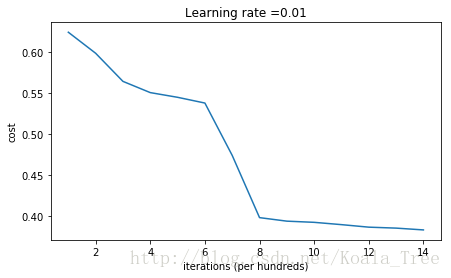
Run the following code to train your model on 15,000 iterations using random initialization.

parameters = model(train_X, train_Y, initialization = "random")
print ("On the train set:")
predictions_train = predict(train_X, train_Y, parameters)
print ("On the test set:")
predictions_test = predict(test_X, test_Y, parameters)

Cost after iteration 0: inf
Cost after iteration 1000: 0.6237287551108738
Cost after iteration 2000: 0.5981106708339466
Cost after iteration 3000: 0.5638353726276827
Cost after iteration 4000: 0.550152614449184
Cost after iteration 5000: 0.5444235275228304
Cost after iteration 6000: 0.5374184054630083
Cost after iteration 7000: 0.47357131493578297
Cost after iteration 8000: 0.39775634899580387
Cost after iteration 9000: 0.3934632865981078
Cost after iteration 10000: 0.39202525076484457
Cost after iteration 11000: 0.38921493051297673
Cost after iteration 12000: 0.38614221789840486
Cost after iteration 13000: 0.38497849983013926
Cost after iteration 14000: 0.38278397192120406

On the train set:
Accuracy: 0.83
On the test set:
Accuracy: 0.86

If you see “inf” as the cost after the iteration 0, this is because of numerical roundoff; a more numerically sophisticated implementation would fix this. But this isn’t worth worrying about for our purposes.

Anyway, it looks like you have broken symmetry, and this gives better results. than before. The model is no longer outputting all 0s.

print (predictions_train)
print (predictions_test)

[[1 0 1 1 0 0 1 1 1 1 1 0 1 0 0 1 0 1 1 0 0 0 1 0 1 1 1 1 1 1 0 1 1 0 0 1 1
  1 1 1 1 1 1 0 1 1 1 1 0 1 0 1 1 1 1 0 0 1 1 1 1 0 1 1 0 1 0 1 1 1 1 0 0 0
  0 0 1 0 1 0 1 1 1 0 0 1 1 1 1 1 1 0 0 1 1 1 0 1 1 0 1 0 1 1 0 1 1 0 1 0 1
  1 0 0 1 0 0 1 1 0 1 1 1 0 1 0 0 1 0 1 1 1 1 1 1 1 0 1 1 0 0 1 1 0 0 0 1 0
  1 0 1 0 1 1 1 0 0 1 1 1 1 0 1 1 0 1 0 1 1 0 1 0 1 1 1 1 0 1 1 1 1 0 1 0 1
  0 1 1 1 1 0 1 1 0 1 1 0 1 1 0 1 0 1 1 1 0 1 1 1 0 1 0 1 0 0 1 0 1 1 0 1 1
  0 1 1 0 1 1 1 0 1 1 1 1 0 1 0 0 1 1 0 1 1 1 0 0 0 1 1 0 1 1 1 1 0 1 1 0 1
  1 1 0 0 1 0 0 0 1 0 0 0 1 1 1 1 0 0 0 0 1 1 1 1 0 0 1 1 1 1 1 1 1 0 0 0 1
  1 1 1 0]]
[[1 1 1 1 0 1 0 1 1 0 1 1 1 0 0 0 0 1 0 1 0 0 1 0 1 0 1 1 1 1 1 0 0 0 0 1 0
  1 1 0 0 1 1 1 1 1 0 1 1 1 0 1 0 1 1 0 1 0 1 0 1 1 1 1 1 1 1 1 1 0 1 0 1 1
  1 1 1 0 1 0 0 1 0 0 0 1 1 0 1 1 0 0 0 1 1 0 1 1 0 0]]

plt.title("Model with large random initialization")
axes = plt.gca()
axes.set_xlim([-1.5,1.5])
axes.set_ylim([-1.5,1.5])
plot_decision_boundary(lambda x: predict_dec(parameters, x.T), train_X, train_Y)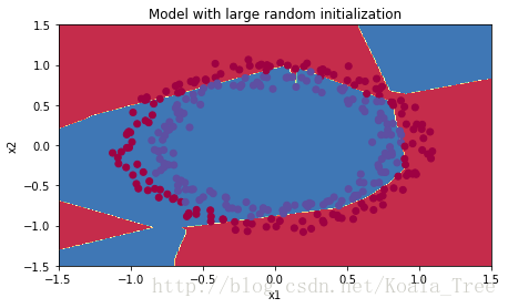

Observations:
- The cost starts very high. This is because with large random-valued weights, the last activation (sigmoid) outputs results that are very close to 0 or 1 for some examples, and when it gets that example wrong it incurs a very high loss for that example. Indeed, when $\log(a^{[3]}) = \log(0)$ , the loss goes to infinity.
- Poor initialization can lead to vanishing/exploding gradients, which also slows down the optimization algorithm.
- If you train this network longer you will see better results, but initializing with overly large random numbers slows down the optimization.

In summary:
- Initializing weights to very large random values does not work well.
- Hopefully intializing with small random values does better. The important question is: how small should be these random values be? Lets find out in the next part!

4 - He initialization

Finally, try “He Initialization”; this is named for the first author of He et al., 2015. (If you have heard of “Xavier initialization”, this is similar except Xavier initialization uses a scaling factor for the weights $W^{[l]}$ of sqrt(1./layers_dims[l-1]) where He initialization would use sqrt(2./layers_dims[l-1]).)

Exercise: Implement the following function to initialize your parameters with He initialization.

Hint: This function is similar to the previous initialize_parameters_random(...). The only difference is that instead of multiplying np.random.randn(..,..) by 10, you will multiply it by $\sqrt{\frac{2}{\text{dimension of the previous layer}}}$ , which is what He initialization recommends for layers with a ReLU activation.

# GRADED FUNCTION: initialize_parameters_he

def initialize_parameters_he(layers_dims):
    """
    Arguments:
    layer_dims -- python array (list) containing the size of each layer.

    Returns:
    parameters -- python dictionary containing your parameters "W1", "b1", ..., "WL", "bL":
                    W1 -- weight matrix of shape (layers_dims[1], layers_dims[0])
                    b1 -- bias vector of shape (layers_dims[1], 1)
                    ...
                    WL -- weight matrix of shape (layers_dims[L], layers_dims[L-1])
                    bL -- bias vector of shape (layers_dims[L], 1)
    """

    np.random.seed(3)
    parameters = {}
    L = len(layers_dims) - 1 # integer representing the number of layers

    for l in range(1, L + 1):
        ### START CODE HERE ### (≈ 2 lines of code)
        parameters['W' + str(l)] = np.random.randn(layers_dims[l],layers_dims[l-1])*np.sqrt(2./layers_dims[l-1])
        parameters['b' + str(l)] = np.zeros((layers_dims[l],1))
        ### END CODE HERE ###

    return parameters

parameters = initialize_parameters_he([2, 4, 1])
print("W1 = " + str(parameters["W1"]))
print("b1 = " + str(parameters["b1"]))
print("W2 = " + str(parameters["W2"]))
print("b2 = " + str(parameters["b2"]))

W1 = [[ 1.78862847  0.43650985]
 [ 0.09649747 -1.8634927 ]
 [-0.2773882  -0.35475898]
 [-0.08274148 -0.62700068]]
b1 = [[ 0.]
 [ 0.]
 [ 0.]
 [ 0.]]
W2 = [[-0.03098412 -0.33744411 -0.92904268  0.62552248]]
b2 = [[ 0.]]

Run the following code to train your model on 15,000 iterations using He initialization.

parameters = model(train_X, train_Y, initialization = "he")
print ("On the train set:")
predictions_train = predict(train_X, train_Y, parameters)
print ("On the test set:")
predictions_test = predict(test_X, test_Y, parameters)

Cost after iteration 0: 0.8830537463419761
Cost after iteration 1000: 0.6879825919728063
Cost after iteration 2000: 0.6751286264523371
Cost after iteration 3000: 0.6526117768893807
Cost after iteration 4000: 0.6082958970572938
Cost after iteration 5000: 0.5304944491717495
Cost after iteration 6000: 0.4138645817071794
Cost after iteration 7000: 0.3117803464844441
Cost after iteration 8000: 0.23696215330322562
Cost after iteration 9000: 0.18597287209206836
Cost after iteration 10000: 0.1501555628037182
Cost after iteration 11000: 0.12325079292273548
Cost after iteration 12000: 0.09917746546525937
Cost after iteration 13000: 0.0845705595402428
Cost after iteration 14000: 0.07357895962677366

On the train set:
Accuracy: 0.993333333333
On the test set:
Accuracy: 0.96

plt.title("Model with He initialization")
axes = plt.gca()
axes.set_xlim([-1.5,1.5])
axes.set_ylim([-1.5,1.5])
plot_decision_boundary(lambda x: predict_dec(parameters, x.T), train_X, train_Y)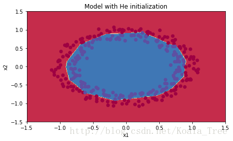

Observations:
- The model with He initialization separates the blue and the red dots very well in a small number of iterations.

5 - Conclusions

You have seen three different types of initializations. For the same number of iterations and same hyperparameters the comparison is:

Model	Train accuracy	Problem/Comment
3-layer NN with zeros initialization	50%	fails to break symmetry
3-layer NN with large random initialization	83%	too large weights
3-layer NN with He initialization	99%	recommended method

What you should remember from this notebook:
- Different initializations lead to different results
- Random initialization is used to break symmetry and make sure different hidden units can learn different things
- Don’t intialize to values that are too large
- He initialization works well for networks with ReLU activations.

Part 2：Regularization

Let’s first import the packages you are going to use.

# import packages
import numpy as np
import matplotlib.pyplot as plt
from reg_utils import sigmoid, relu, plot_decision_boundary, initialize_parameters, load_2D_dataset, predict_dec
from reg_utils import compute_cost, predict, forward_propagation, backward_propagation, update_parameters
import sklearn
import sklearn.datasets
import scipy.io
from testCases import *

%matplotlib inline
plt.rcParams['figure.figsize'] = (7.0, 4.0) # set default size of plots
plt.rcParams['image.interpolation'] = 'nearest'
plt.rcParams['image.cmap'] = 'gray'

There are some function iported：

def initialize_parameters(layer_dims):
    """
    Arguments:
    layer_dims -- python array (list) containing the dimensions of each layer in our network

    Returns:
    parameters -- python dictionary containing your parameters "W1", "b1", ..., "WL", "bL":
                    W1 -- weight matrix of shape (layer_dims[l], layer_dims[l-1])
                    b1 -- bias vector of shape (layer_dims[l], 1)
                    Wl -- weight matrix of shape (layer_dims[l-1], layer_dims[l])
                    bl -- bias vector of shape (1, layer_dims[l])

    Tips:
    - For example: the layer_dims for the "Planar Data classification model" would have been [2,2,1]. 
    This means W1's shape was (2,2), b1 was (1,2), W2 was (2,1) and b2 was (1,1). Now you have to generalize it!
    - In the for loop, use parameters['W' + str(l)] to access Wl, where l is the iterative integer.
    """

    np.random.seed(3)
    parameters = {}
    L = len(layer_dims) # number of layers in the network

    for l in range(1, L):
        parameters['W' + str(l)] = np.random.randn(layer_dims[l], layer_dims[l-1]) / np.sqrt(layer_dims[l-1])
        parameters['b' + str(l)] = np.zeros((layer_dims[l], 1))

        assert(parameters['W' + str(l)].shape == layer_dims[l], layer_dims[l-1])
        assert(parameters['W' + str(l)].shape == layer_dims[l], 1)


    return parameters


def compute_cost(a3, Y):
    """
    Implement the cost function

    Arguments:
    a3 -- post-activation, output of forward propagation
    Y -- "true" labels vector, same shape as a3

    Returns:
    cost - value of the cost function
    """
    m = Y.shape[1]

    logprobs = np.multiply(-np.log(a3),Y) + np.multiply(-np.log(1 - a3), 1 - Y)
    cost = 1./m * np.nansum(logprobs)

    return cost


def load_2D_dataset():
    data = scipy.io.loadmat('datasets/data.mat')
    train_X = data['X'].T
    train_Y = data['y'].T
    test_X = data['Xval'].T
    test_Y = data['yval'].T

    plt.scatter(train_X[0, :], train_X[1, :], c=train_Y, s=40, cmap=plt.cm.Spectral);

    return train_X, train_Y, test_X, test_Y

The data set in load_2D_dataset() ,you can get it in the address : http://pan.baidu.com/s/1sl4YzfB . If the link is invalid , please leave your message in the message area.

Problem Statement: You have just been hired as an AI expert by the French Football Corporation. They would like you to recommend positions where France’s goal keeper should kick the ball so that the French team’s players can then hit it with their head.

Figure 1 : Football field
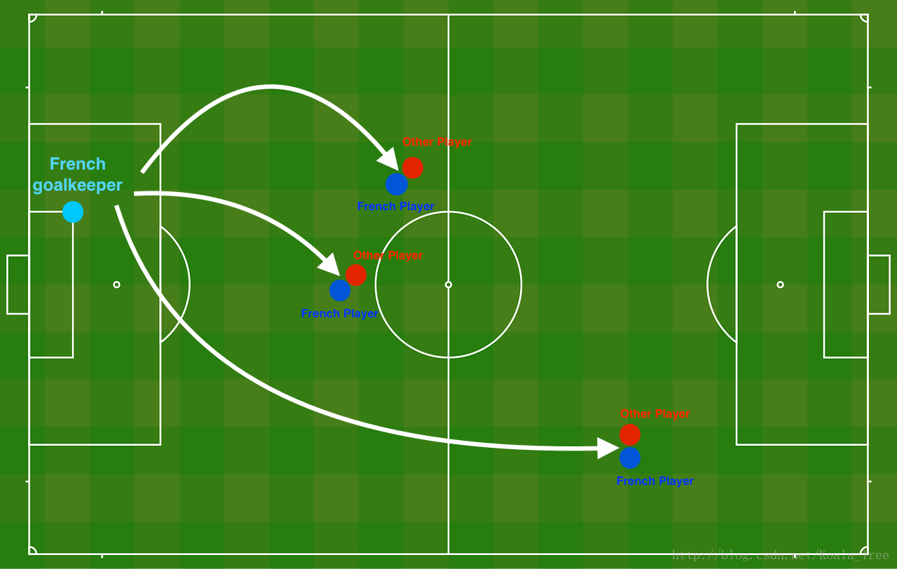
The goal keeper kicks the ball in the air, the players of each team are fighting to hit the ball with their head

They give you the following 2D dataset from France’s past 10 games.

train_X, train_Y, test_X, test_Y = load_2D_dataset()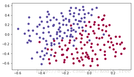

Each dot corresponds to a position on the football field where a football player has hit the ball with his/her head after the French goal keeper has shot the ball from the left side of the football field.
- If the dot is blue, it means the French player managed to hit the ball with his/her head
- If the dot is red, it means the other team’s player hit the ball with their head

Your goal: Use a deep learning model to find the positions on the field where the goalkeeper should kick the ball.

Analysis of the dataset: This dataset is a little noisy, but it looks like a diagonal line separating the upper left half (blue) from the lower right half (red) would work well.

You will first try a non-regularized model. Then you’ll