MATLAB 决策树工具箱

Train Decision Trees Using Classification Learner App

---

This example shows how to create and compare various classification trees using Classification Learner, and export trained models to the workspace to make predictions for new data.

You can train classification trees to predict responses to data. To predict a response, follow the decisions in the tree from the root (beginning) node down to a leaf node. The leaf node contains the response.

Statistics and Machine Learning Toolbox™ trees are binary. Each step in a prediction involves checking the value of one predictor (variable). For example, here is a simple classification tree:

This tree predicts classifications based on two predictors, x1 and x2. To predict, start at the top node. At each decision, check the values of the predictors to decide which branch to follow. When the branches reach a leaf node, the data is classified either as type 0 or 1.

1. In MATLAB®, load the fisheriris data set and create a table of measurement predictors (or features) using variables from the data set to use for a classification.

fishertable = readtable('fisheriris.csv');

1. On the Apps tab, in the Machine Learning and Deep Learning group, click Classification Learner.
2. On the Classification Learner tab, in the File section, click New Session > From Workspace.

1. In the New Session dialog box, select the table fishertable from the Data Set Variable list (if necessary).

Observe that the app has selected response and predictor variables based on their data type. Petal and sepal length and width are predictors, and species is the response that you want to classify. For this example, do not change the selections.

1. To accept the default validation scheme and continue, click Start Session. The default validation option is cross-validation, to protect against overfitting.

Classification Learner creates a scatter plot of the data.

1. Use the scatter plot to investigate which variables are useful for predicting the response. Select different options on the X and Y lists under Predictors to visualize the distribution of species and measurements. Observe which variables separate the species colors most clearly.

Observe that the setosa species (blue points) is easy to separate from the other two species with all four predictors. The versicolor and virginica species are much closer together in all predictor measurements, and overlap especially when you plot sepal length and width. setosa is easier to predict than the other two species.

1. To create a classification tree model, on the Classification Learner tab, in the Model Type section, click the down arrow to expand the gallery and click Coarse Tree. Then click Train.

Tip

If you have Parallel Computing Toolbox™ then the first time you click Train you see a dialog while the app opens a parallel pool of workers. After the pool opens, you can train multiple classifiers at once and continue working.

The app creates a simple classification tree, and plots the results.

Observe the Coarse Tree model in the History list. Check the model validation score in the Accuracy box. The model has performed well.

Note

With validation, there is some randomness in the results, so your model validation score results can vary from those shown.

1. Examine the scatter plot. An X indicates misclassified points. The blue points (setosa species) are all correctly classified, but some of the other two species are misclassified. Under Plot, switch between the Data and Model Predictions options. Observe the color of the incorrect (X) points. Alternatively, while plotting model predictions, to view only the incorrect points, clear the Correct check box.
2. Train a different model to compare. Click Medium Tree, and then click Train.

When you click Train, the app displays a new model in the History list.

1. Observe the Medium Tree model in the History list. The model validation score is no better than the coarse tree score. The app outlines in a box the Accuracy score of the best model. Click each model in the History list to view and compare the results.
2. Examine the scatter plot for the Medium Tree model. The medium tree classifies as many points correctly as the previous coarse tree. You want to avoid overfitting, and the coarse tree performs well, so base all further models on the coarse tree.
3. Select Coarse Tree in the History list. To try to improve the model, try including different features in the model. See if you can improve the model by removing features with low predictive power.

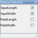
On the Classification Learner tab, in the Features section, click Feature Selection.

In the Feature Selection dialog box, clear the check boxes for PetalLength and PetalWidth to exclude them from the predictors. A new draft model appears in the model history list with your new settings 2/4 features, based on the coarse tree.

Click Train to train a new tree model using the new predictor options.

1. Observe the third model in the History list. It is also a Coarse Tree model, trained using only 2 of 4 predictors. The History list displays how many predictors are excluded. To check which predictors are included, click a model in the History list and observe the check boxes in the Feature Selection dialog box. The model with only sepal measurements has a much lower accuracy score than the petals-only model.
2. Train another model including only the petal measurements. Change the selections in the Feature Selection dialog box and click Train.

The model trained using only petal measurements performs comparably to the models containing all predictors. The models predict no better using all the measurements compared to only the petal measurements. If data collection is expensive or difficult, you might prefer a model that performs satisfactorily without some predictors.

1. Repeat to train two more models including only the width measurements and then the length measurements. There is not much difference in score between several of the models.
2. Choose a best model among those of similar scores by examining the performance in each class. Select the coarse tree that includes all the predictors. To inspect the accuracy of the predictions in each class, on the Classification Learner tab, in the Plots section, click Confusion Matrix. Use this plot to understand how the currently selected classifier performed in each class. View the matrix of true class and predicted class results.

Look for areas where the classifier performed poorly by examining cells off the diagonal that display high numbers and are red. In these red cells, the true class and the predicted class do not match. The data points are misclassified.

Note

With validation, there is some randomness in the results, so your confusion matrix results can vary from those shown.

In this figure, examine the third cell in the middle row. In this cell, true class is versicolor, but the model misclassified the points as virginica. For this model, the cell shows 4 misclassified (your results can vary). To view percentages instead of numbers of observations, select the True Positive Rates option under Plot controls..

You can use this information to help you choose the best model for your goal. If false positives in this class are very important to your classification problem, then choose the best model at predicting this class. If false positives in this class are not very important, and models with fewer predictors do better in other classes, then choose a model to tradeoff some overall accuracy to exclude some predictors and make future data collection easier.

1. Compare the confusion matrix for each model in the History list. Check the Feature Selection dialog box to see which predictors are included in each model.
2. To investigate features to include or exclude, use the scatter plot and the parallel coordinates plot. On the Classification Learner tab, in the Plots section, click Parallel Coordinates Plot. You can see that petal length and petal width are the features that separate the classes best.

1. To learn about model settings, choose a model in the History list and view the advanced settings. The nonoptimizable model options in the Model Type gallery are preset starting points, and you can change further settings. On the Classification Learner tab, in the Model Type section, click Advanced. Compare the simple and medium tree models in the history, and observe the differences in the Advanced Tree Options dialog box. The Maximum Number of Splits setting controls tree depth.

To try to improve the coarse tree model further, try changing the Maximum Number of Splits setting, then train a new model by clicking Train.

View the settings for the selected trained model in the Current model pane, or in the Advanced dialog box.

1. To export the best trained model to the workspace, on the Classification Learner tab, in the Export section, click Export Model. In the Export Model dialog box, click OK to accept the default variable name trainedModel.

Look in the command window to see information about the results.

1. To visualize your decision tree model, enter:

view(trainedModel.ClassificationTree,'Mode','graph')

1. You can use the exported classifier to make predictions on new data. For example, to make predictions for the fishertable data in your workspace, enter:

yfit = trainedModel.predictFcn(fishertable)

The output yfit contains a class prediction for each data point.

1. If you want to automate training the same classifier with new data, or learn how to programmatically train classifiers, you can generate code from the app. To generate code for the best trained model, on the Classification Learner tab, in the Export section, click Generate Function.

The app generates code from your model and displays the file in the MATLAB Editor. To learn more, see Generate MATLAB Code to Train the Model with New Data.

This example uses Fisher's 1936 iris data. The iris data contains measurements of flowers: the petal length, petal width, sepal length, and sepal width for specimens from three species. Train a classifier to predict the species based on the predictor measurements.

Use the same workflow to evaluate and compare the other classifier types you can train in Classification Learner.

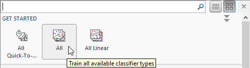
To try all the nonoptimizable classifier model presets available for your data set:

1. Click the arrow on the far right of the Model Type section to expand the list of classifiers.
2. Click All, then click Train.

To learn about other classifier types, see Train Classification Models in Classification Learner App.

原文地址：Train Decision Trees Using Classification Learner App- MATLAB & Simulink