RNN和LSTM的正向/前向传播-图示公式和代码

本文链接：https://blog.csdn.net/liangyihuai/article/details/89526121

本文先讲的基础版本的RNN，包含内部结构示意图，公式以及每一步的python代码实现。然后，拓展到LSTM的前向传播网络。结合图片+公式+可运行的代码，清晰充分明白RNN的前向传播网络的具体过程。完整的可执行的代码见文末。

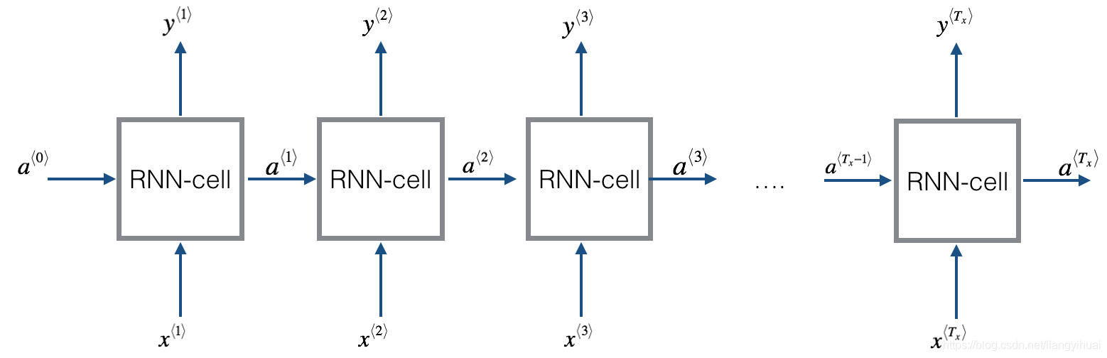
下面图片是RNN网络的整体示意图。每一个方框是“同一个节点处的不同时间点的表示“。也就是RNN-cell都是同一个，只是时间点不一样，所以展开画出来。所以，它们共用相同的”可训练/可学习“参数，该参数在下面的公式中表示为W和b。
在这里插入图片描述

下图是表示上图中的一个RNN-cell。其中可训练的参数为 $W_{ax}$ 、 $W_{aa}$ 、 $b_{a}$ 、 $W_{ya}$ 、 $b_{b}$ ，其中 $a^{<t>}$ 表示网络的隐藏状态。
在这里插入图片描述
如果把上面的cell按照时间的前后顺序连接起来，那么就变成了下图所示的样子了。在该RNN中，输入数据和输出数据是什么样子的呢？比如可以把一条句子作为一个输入数据。那么这个句子可以表示为[ $x^{<1>}$ , $x^{<2>}$ , $x^{<>}$ ,… $x^{<T>}$ ]，其中 $x^{<i>}$ 表示一个单词。需要注意的是， $x^{<i>}$ 可能是一个向量，比如在使用one-hot表示一个单词的时候。
在这里插入图片描述
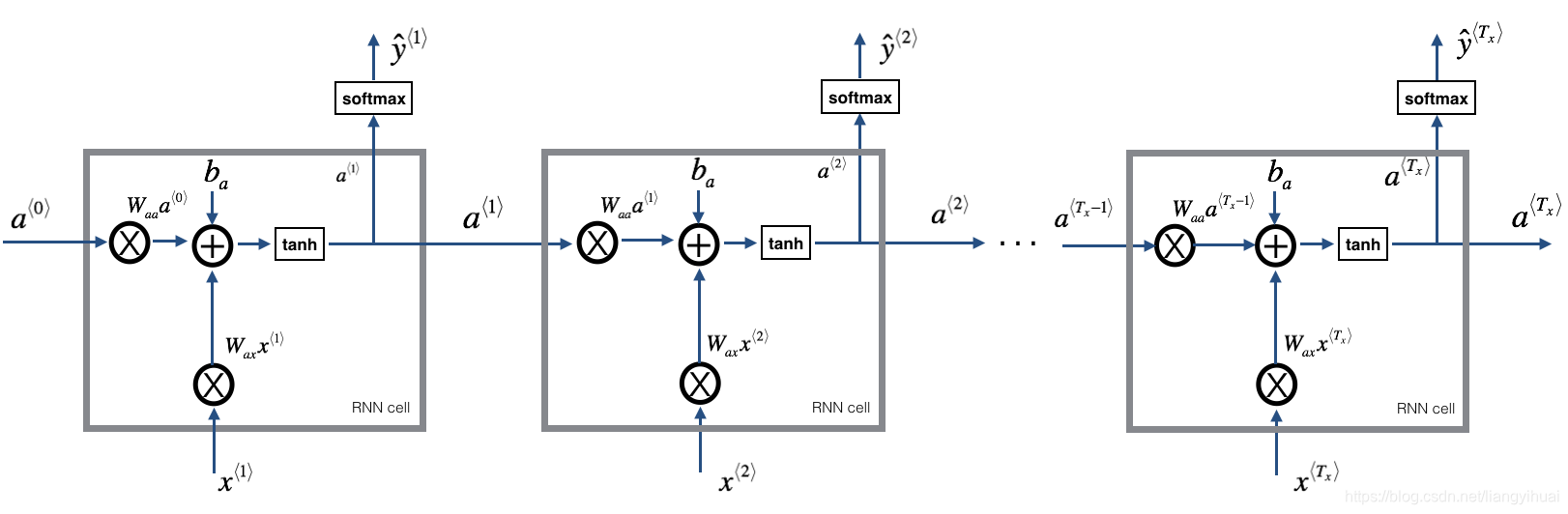
下面，我们使用代码来实现上面图示的部分。下面代码分为2部分，第一部分为上面第二张图片的代码实现，表示单个cell的前向传播。第二部分为把多个cell连起来之后的前向传播，对应上面的第三个图片。

下面代码表示单个cell的前向传播

import numpy as np
from rnn_utils import *

# GRADED FUNCTION: rnn_cell_forward

def rnn_cell_forward(xt, a_prev, parameters):
    """
    Implements a single forward step of the RNN-cell as described in Figure (2)

    Arguments:
    xt -- your input data at timestep "t", numpy array of shape (n_x, m).
    a_prev -- Hidden state at timestep "t-1", numpy array of shape (n_a, m)
    parameters -- python dictionary containing:
                        Wax -- Weight matrix multiplying the input, numpy array of shape (n_a, n_x)
                        Waa -- Weight matrix multiplying the hidden state, numpy array of shape (n_a, n_a)
                        Wya -- Weight matrix relating the hidden-state to the output, numpy array of shape (n_y, n_a)
                        ba --  Bias, numpy array of shape (n_a, 1)
                        by -- Bias relating the hidden-state to the output, numpy array of shape (n_y, 1)
    Returns:
    a_next -- next hidden state, of shape (n_a, m)
    yt_pred -- prediction at timestep "t", numpy array of shape (n_y, m)
    cache -- tuple of values needed for the backward pass, contains (a_next, a_prev, xt, parameters)
    """
    
    # Retrieve parameters from "parameters"
    Wax = parameters["Wax"]
    Waa = parameters["Waa"]
    Wya = parameters["Wya"]
    ba = parameters["ba"]
    by = parameters["by"]
    
    ### START CODE HERE ### (≈2 lines)
    # compute next activation state using the formula given above
    a_next = np.tanh(np.dot(Wax, xt) + np.dot(Waa, a_prev) + ba)
    # compute output of the current cell using the formula given above
    yt_pred = softmax(np.dot(Wya, a_next) + by)   
    ### END CODE HERE ###
    
    # store values you need for backward propagation in cache
    cache = (a_next, a_prev, xt, parameters)
    
    return a_next, yt_pred, cache

下面代码表示多个cell连接之后的前向传播，

# GRADED FUNCTION: rnn_forward

def rnn_forward(x, a0, parameters):
    """
    Implement the forward propagation of the recurrent neural network described in Figure (3).

    Arguments:
    x -- Input data for every time-step, of shape (n_x, m, T_x).
    a0 -- Initial hidden state, of shape (n_a, m)
    parameters -- python dictionary containing:
                        Waa -- Weight matrix multiplying the hidden state, numpy array of shape (n_a, n_a)
                        Wax -- Weight matrix multiplying the input, numpy array of shape (n_a, n_x)
                        Wya -- Weight matrix relating the hidden-state to the output, numpy array of shape (n_y, n_a)
                        ba --  Bias numpy array of shape (n_a, 1)
                        by -- Bias relating the hidden-state to the output, numpy array of shape (n_y, 1)

    Returns:
    a -- Hidden states for every time-step, numpy array of shape (n_a, m, T_x)
    y_pred -- Predictions for every time-step, numpy array of shape (n_y, m, T_x)
    caches -- tuple of values needed for the backward pass, contains (list of caches, x)
    """
    
    # Initialize "caches" which will contain the list of all caches
    caches = []
    
    # Retrieve dimensions from shapes of x and parameters["Wya"]
    n_x, m, T_x = x.shape
    n_y, n_a = parameters["Wya"].shape
    
    ### START CODE HERE ###
    
    # initialize "a" and "y" with zeros (≈2 lines)
    a = np.zeros((n_a, m, T_x))
    y_pred = np.zeros((n_y, m, T_x))
    
    # Initialize a_next (≈1 line)
    a_next = a0
    
    # loop over all time-steps
    for t in range(T_x):
        # Update next hidden state, compute the prediction, get the cache (≈1 line)
        a_next, yt_pred, cache = rnn_cell_forward(x[:, :, t], a_next, parameters)
        # Save the value of the new "next" hidden state in a (≈1 line)
        a[:,:,t] = a_next
        # Save the value of the prediction in y (≈1 line)
        y_pred[:,:,t] = yt_pred
        # Append "cache" to "caches" (≈1 line)
        caches += cache
        
    ### END CODE HERE ###
    
    # store values needed for backward propagation in cache
    caches = (caches, x)
    
    return a, y_pred, caches

第二部分：Long Short-Term Memory (LSTM)

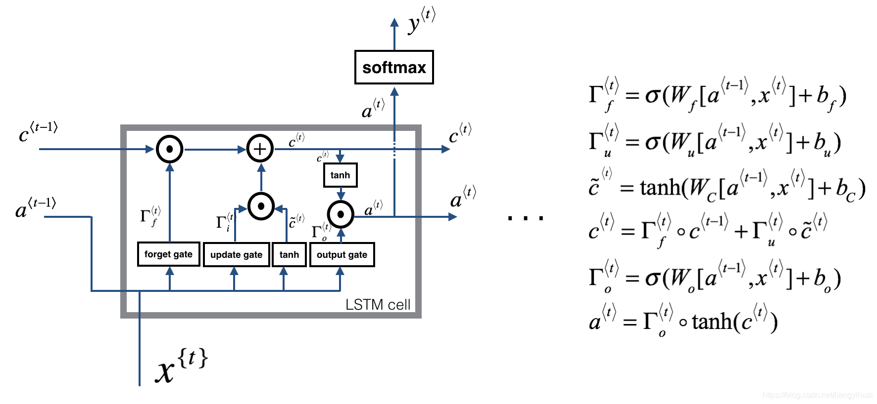
LSTM是RNN网络的一种，是目前常用的RNN变种。下面讲的是LSTM网络的前向传播。下图左边表示网络中一个cell内部示意图，右边表示它的公式了。
在这里插入图片描述
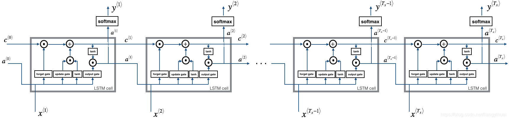
如果把上图的cell按照不同的时间点连接在一起，就变成了下图的样子了。结构上和基础版本的RNN是一样的。

LSTM跟基本的RNN不一样的地方在于，它多了三个门，分别是忘记门，更新门和输出门。它们的作用是解决因为梯度消失而导致的长依赖问题，让网络能够记住相对远的历史信息。所谓的门，表示的是在（0，1）之间的值，可以类比数字电路，如果值越接近1，表示门的打开程度越大，如果值越接近0，表示门越处于关闭状态。所以，我们使用sigmoid函数来构造门。下面给出三个门的公式，仔细观察，发现三个公式的结构是一样的，只是都是通过 $a^{\langle t-1 \rangle}, x^{\{t\}}$ 这两个数值来构造，并且都有各自的W和b学习参数。

忘记门（forget gate）： $\Gamma_f^{\langle t \rangle} = \sigma(W_f[a^{\langle t-1 \rangle}, x^{\langle t \rangle}] + b_f)\tag{1}$

更新门（update gate）： $\Gamma_u^{\langle t \rangle} = \sigma(W_u[a^{\langle t-1 \rangle}, x^{\{t\}}] + b_u)\tag{2}$

输出门（output gate）： $\Gamma_o^{\langle t \rangle}= \sigma(W_o[a^{\langle t-1 \rangle}, x^{\langle t \rangle}] + b_o)\tag{5}$

带波浪线的 $\tilde{c}^{<t>}$ 表示的是一个临时变量，我们的目的是通过 $\tilde{c}^{<t>}$ 来构造 ${c}^{<t>}$ ，而 ${c}^{<t>}$ 在LSTM中的作用是作为额外的记忆单元，不同于隐藏状态 $a$ ， ${c}^{<t>}$ 的目的是记忆。，

$\tilde{c}^{\langle t \rangle} = \tanh(W_c[a^{\langle t-1 \rangle}, x^{\langle t \rangle}] + b_c)\tag{3}$

既然 ${c}^{<t>}$ 是为了记忆网络中的历史信息，那么就存在让这个记忆单元忘记没用的旧数据，以及添加（更新）有用的新数据的能力。所以就有了忘记门和更新门。下面公式中，注意两个门的作用对象是不一样的，忘记门作用于历史的记忆状态，而更新门作用于当前的记忆状态。

$c^{\langle t \rangle} = \Gamma_f^{\langle t \rangle}* c^{\langle t-1 \rangle} + \Gamma_u^{\langle t \rangle} *\tilde{c}^{\langle t \rangle} \tag{4}$

从下面的公式中，输出门作用于记忆单元，控制记忆单元的向外输出量。

$a^{\langle t \rangle} = \Gamma_o^{\langle t \rangle}* \tanh(c^{\langle t \rangle})\tag{6}$

最终，网络的最终输出公式为：
$\hat{y}^{\langle t \rangle} = softmax(W_{ya} a^{\langle t \rangle} + b_y)$

下面代码实现LSTM中一个cell的功能，对应LSTM部分的第一个图片

# GRADED FUNCTION: lstm_cell_forward

def lstm_cell_forward(xt, a_prev, c_prev, parameters):
    """
    Implement a single forward step of the LSTM-cell as described in Figure (4)

    Arguments:
    xt -- your input data at timestep "t", numpy array of shape (n_x, m).
    a_prev -- Hidden state at timestep "t-1", numpy array of shape (n_a, m)
    c_prev -- Memory state at timestep "t-1", numpy array of shape (n_a, m)
    parameters -- python dictionary containing:
                        Wf -- Weight matrix of the forget gate, numpy array of shape (n_a, n_a + n_x)
                        bf -- Bias of the forget gate, numpy array of shape (n_a, 1)
                        Wi -- Weight matrix of the update gate, numpy array of shape (n_a, n_a + n_x)
                        bi -- Bias of the update gate, numpy array of shape (n_a, 1)
                        Wc -- Weight matrix of the first "tanh", numpy array of shape (n_a, n_a + n_x)
                        bc --  Bias of the first "tanh", numpy array of shape (n_a, 1)
                        Wo -- Weight matrix of the output gate, numpy array of shape (n_a, n_a + n_x)
                        bo --  Bias of the output gate, numpy array of shape (n_a, 1)
                        Wy -- Weight matrix relating the hidden-state to the output, numpy array of shape (n_y, n_a)
                        by -- Bias relating the hidden-state to the output, numpy array of shape (n_y, 1)
                        
    Returns:
    a_next -- next hidden state, of shape (n_a, m)
    c_next -- next memory state, of shape (n_a, m)
    yt_pred -- prediction at timestep "t", numpy array of shape (n_y, m)
    cache -- tuple of values needed for the backward pass, contains (a_next, c_next, a_prev, c_prev, xt, parameters)
    
    Note: ft/it/ot stand for the forget/update/output gates, cct stands for the candidate value (c tilde),
          c stands for the memory value
    """

    # Retrieve parameters from "parameters"
    Wf = parameters["Wf"]
    bf = parameters["bf"]
    Wi = parameters["Wi"]
    bi = parameters["bi"]
    Wc = parameters["Wc"]
    bc = parameters["bc"]
    Wo = parameters["Wo"]
    bo = parameters["bo"]
    Wy = parameters["Wy"]
    by = parameters["by"]
    
    # Retrieve dimensions from shapes of xt and Wy
    n_x, m = xt.shape
    n_y, n_a = Wy.shape

    ### START CODE HERE ###
    # Concatenate a_prev and xt (≈3 lines)
    concat = np.zeros((n_x + n_a, m))
    concat[: n_a, :] = a_prev
    concat[n_a :, :] = xt

    # Compute values for ft, it, cct, c_next, ot, a_next using the formulas given figure (4) (≈6 lines)
    ft = sigmoid(np.dot(Wf, concat) + bf)
    it = sigmoid(np.dot(Wi, concat) + bi)
    cct = np.tanh(np.dot(Wc, concat) + bc)
    c_next = ft * c_prev + it * cct
    ot = sigmoid(np.dot(Wo, concat) + bo)
    a_next = ot * np.tanh(c_next)
    
    # Compute prediction of the LSTM cell (≈1 line)
    yt_pred = softmax(np.dot(Wy, a_next) + by)
    ### END CODE HERE ###

    # store values needed for backward propagation in cache
    cache = (a_next, c_next, a_prev, c_prev, ft, it, cct, ot, xt, parameters)

    return a_next, c_next, yt_pred, cache

下面代码实现LSTM中连接多个cell的功能，对应LSTM部分的第2个图片

# GRADED FUNCTION: lstm_forward

def lstm_forward(x, a0, parameters):
    """
    Implement the forward propagation of the recurrent neural network using an LSTM-cell described in Figure (3).

    Arguments:
    x -- Input data for every time-step, of shape (n_x, m, T_x).
    a0 -- Initial hidden state, of shape (n_a, m)
    parameters -- python dictionary containing:
                        Wf -- Weight matrix of the forget gate, numpy array of shape (n_a, n_a + n_x)
                        bf -- Bias of the forget gate, numpy array of shape (n_a, 1)
                        Wi -- Weight matrix of the update gate, numpy array of shape (n_a, n_a + n_x)
                        bi -- Bias of the update gate, numpy array of shape (n_a, 1)
                        Wc -- Weight matrix of the first "tanh", numpy array of shape (n_a, n_a + n_x)
                        bc -- Bias of the first "tanh", numpy array of shape (n_a, 1)
                        Wo -- Weight matrix of the output gate, numpy array of shape (n_a, n_a + n_x)
                        bo -- Bias of the output gate, numpy array of shape (n_a, 1)
                        Wy -- Weight matrix relating the hidden-state to the output, numpy array of shape (n_y, n_a)
                        by -- Bias relating the hidden-state to the output, numpy array of shape (n_y, 1)
                        
    Returns:
    a -- Hidden states for every time-step, numpy array of shape (n_a, m, T_x)
    y -- Predictions for every time-step, numpy array of shape (n_y, m, T_x)
    caches -- tuple of values needed for the backward pass, contains (list of all the caches, x)
    """

    # Initialize "caches", which will track the list of all the caches
    caches = []
    
    ### START CODE HERE ###
    # Retrieve dimensions from shapes of x and Wy (≈2 lines)
    n_x, m, T_x = x.shape
    n_y, n_a = parameters["Wy"].shape
    
    # initialize "a", "c" and "y" with zeros (≈3 lines)
    a = np.zeros((n_a, m, T_x))
    c = np.zeros((n_a, m, T_x))
    y = np.zeros((n_y, m, T_x))
    
    # Initialize a_next and c_next (≈2 lines)
    a_next = a0
    c_next = np.zeros(a_next.shape)
    
    # loop over all time-steps
    for t in range(T_x):
        # Update next hidden state, next memory state, compute the prediction, get the cache (≈1 line)
        a_next, c_next, yt, cache = lstm_cell_forward(x[:, :, t], a_next, c_next, parameters)
        # Save the value of the new "next" hidden state in a (≈1 line)
        a[:,:,t] = a_next
        # Save the value of the prediction in y (≈1 line)
        y[:,:,t] = yt
        # Save the value of the next cell state (≈1 line)
        c[:,:,t]  = c_next
        # Append the cache into caches (≈1 line)
        caches.append(cache)
        
    ### END CODE HERE ###
    
    # store values needed for backward propagation in cache
    caches = (caches, x)

    return a, y, c, caches

完整的可执行的代码：https://github.com/liangyihuai/deeplearning_liang/tree/master/src/rnn/forward_propagation

总结：
本文讲了基础版本的RNN以及LSTM的前向传播算法，结合图片，公式和代码，提供一个全面的通俗易懂的展示。本文没有涉及到RNN网络的反向传播，因为现在的深度学习框架都自动完成了反向传播的功能，在使用的时候，我们只需要关注前向传播，另外，该文章的内容参考了吴恩达老师深度学习课程中的内容。谢谢