第J3周：DenseNet算法实战与解析_densenet代码实现-CSDN博客

本文链接：https://blog.csdn.net/lihuhelihu/article/details/139298088

>本文为[🔗365天深度学习训练营](https://mp.weixin.qq.com/s/rbOOmire8OocQ90QM78DRA) 中的学习记录博客**
> 原作者：[K同学啊 | 接辅导、项目定制](https://mtyjkh.blog.csdn.net/)**

我的环境：
系统环境：win10
语言环境：Python3.9.13
编译器：jupyter notebook
深度学习环境：Pytorch 2.3.0+cpu，torchvision 0.18.0+cpu

一、densenet模型介绍
1、前言
在计算机视觉领域，卷积神经网络(CNN)已经成为最主流的方法，比如GoogLenet，VGG-16Incepetion等模型。CNN史上的一个里程碑事件是ResNet模型的出现，ResNet可以训练出更深的CNN模型，从而实现更高的准确度。ResNet模型的核心是通过建立前面层与后面层之间的“短路连接(shortcuts，skip connection)，进而训练出更深的CNN网络。
今天我们要介绍的是DenseNet模型，它的基本思路与ResNet一致，但是它建立的是前面所有层与后面层的密集连接(dense connection)，它的名称也是由此而来。DenseNet的另一大特色是通过特征在channel上的连接来实现特征重用(feature reuse)。这些特点让DenseNet在参数和计算成本更少的情形下实现比ResNet更优的性能，DenseNet也因此斩获CVPR 2017的最佳论文奖。

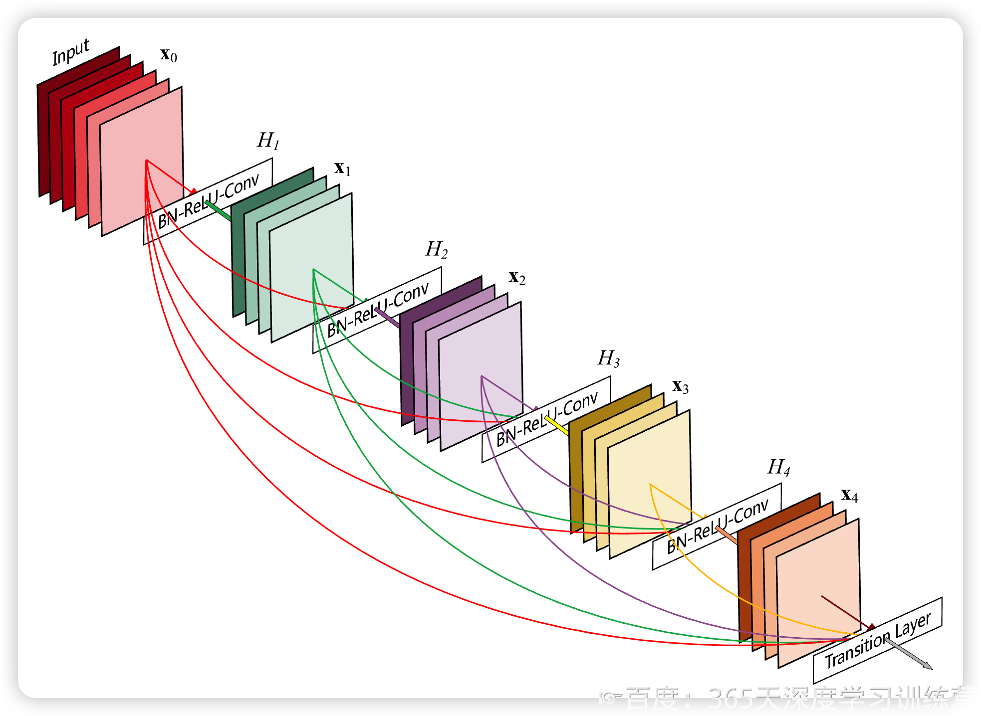图1 Dense模块（5-layer，growth rate of k=4）

2、设计理念
相比ResNet，DenseNet提出了一个更激进的密集连接机制:即互相连接所有的层，具体来说就是每个层都会接受其前面所有层作为其额外的输入。
图3为ResNet网络的残差连接机制，作为对比，图4为DenseNet的密集连接机制。可以看到，ResNet是每个层与前面的某层(一般是2~4层)短路连接在一起，连接方式是通过**元素相加**。而在DenseNet中，每个层都会与前面所有层在channel维度上连接(concat)在一起(即**元素叠加**)，并作为下一层的输入。
对于一个L层的网络，DenseNet共包含 $\tfrac{L(L+1)}2{}$ 个连接，相比ResNet，这是一种密集连接。而且DenseNet是直接concat来自不同层的特征图，这可以实现特征重用，提升效率，这一特点是DenseNet与ResNet最主要的区别。

图2 标准的神经网络传播过程

* 输入和输出的公式是 $X_{l}=H_{l}(X_{l-1})$ ，其中 $H_{l}$ 是一个组合函数，通常包括 BN、ReLU、Pooling、Conv操作， $X_{l-1}$ 是第 $l$ 层输入的特征图， $X_{l}$ 是第 $l$ 层输出的特征图。

图3 ResNet网络的短路连接机制（其中+代表的是元素级相加操作）

* ResNet是跨层相加，输入和输出的公式是 $X_{l}=H_{l}(X_{l-1})+X_{l-1}$

图4 DenseNet 网络的密集连接机制（其中c代表的是channel级连接操作）

* 而对于DesNet，则是采用跨通道concat的形式来连接，会连接前面所有层作为输入，输入和输出的公式是 $X_{l}=H_{l}(X_{0},X_{1},...,X_{l-1})$ 。这里要注意所有的层的输入都来源于前面所有层在channel维度的concat。

3、网络结构

具体介绍网络的具体实现细节如图5所示。

图5 DenseNet的网络结构

CNN网络一般要经过Pooling或者stride>1的Conv来降低特征图的大小，而DenseNet的密集连接方式需要特征图大小保持一致。为了解决这个问题，DenseNet网络中使用DenseBlock+Transition的结构，其中DenseBlock是包含很多层的模块，每个层的特征图大小相同，层与层之间采用密集连接方式。而Transition层是连接两个相邻的DenseBlock，并且通过Pooling使特征图大小降低。图6给出了DenseNet的网路结构，它共包含4个DenseBlock，各个DenseBlock之间通过Transition层连接在一起。

图6 使用DenseBlock+Transition的DenseNet网络

在DenseBlock中，各个层的特征图大小一致，可以在channel维度上连接。DenseBlock中的非线性组合函数 H(·)的是 BN+ReLU+3x3Conv 的结构，如图7所示。另外值得注意的一点是，与ResNet不同，所有DenseBlock中各个层卷积之后均输出k个特征图，即得到的特征图的channel数为k，或者说采用个卷积核。k在DenseNet称为growthrate，这是一个超参数。一般情况下使用较小的k(比如12)，就可以得到较佳的性能。假定输入层的特征图的channel数为 $k_{0}$ ，那么 $l$ 层输入的channel数为 $k_{0}+k_{1,2,...,l-1}$ ，因此随着层数增加，尽管 $k$ 设定得较小，DenseBlock的输入会非常多，不过这是由于特征重用所造成的，每个层仅有 $k$ 个特征是自己独有的。

图7 DenseBlock中的非线性转换结构

由于后面层的输入会非常大，DenseBlock内部可以采用bottleneck层来减少计算量，主要是原有的结构中增加1x1Conv，如图8所示，即BN+ReLU+1x1ConV+BN+ReLU+3x3Conv，称为DenseNet-B结构。其中1x1Conv得到 4 $k$ 个特征图，它起到的作用是降低特征数量，从而提升计算效率。

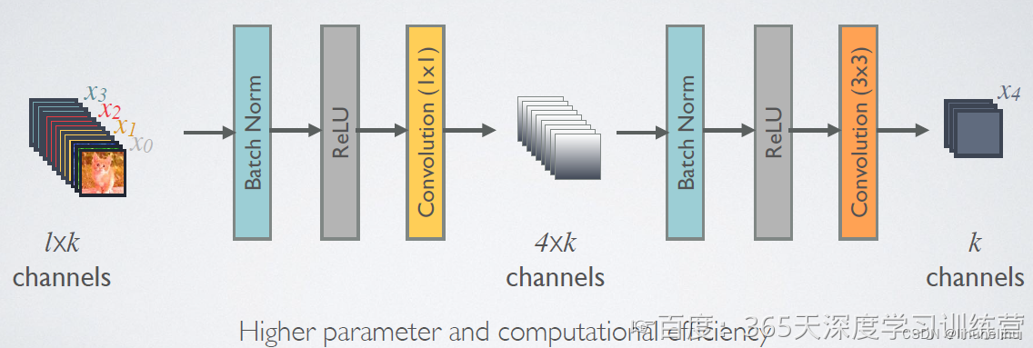图8 使用bottleneck层的DenseBlock结构

对于Transition层，它主要是连接两个相邻的DenseBlock，并且降低特征图大小。Transition层包括一个1x1的卷积和2x2的AvgPooling，结构为BN+ReLU+1x1Conv+2x2AvgPooling。另外，Transition层可以起到压缩模型的作用。假定Transition层的上接DenseBlock得到的特征图channels数为 $m$ ，Transition层可以产生 $\left \lfloor \theta m \right \rfloor$ 个特征(通过卷积层)，其中 $\theta \in (0,1)$ 是压缩系数(compressionrate)。当 $\theta =1$ 时，特征个数经过Transition层没有变化，即无压缩，而当压缩系数小于1时，这种结构称为DenseNet-C，文中使用 $\theta =0.5$ 。对于使用bottleneck层的DenseBlock结构和压缩系数小于1的Transition组合结构称为DenseNet-BC。
对于lmageNet数据集，图片输入大小为224x224，网络结构采用包含4个DenseBlock的DenseNet-BC，其首先是一个stride=2的7x7卷积层，然后是一个stride=2的3x3 MaxPooling层，后面才进入DenseBlock。lmageNet数据集所采用的网络配置如表1所示：

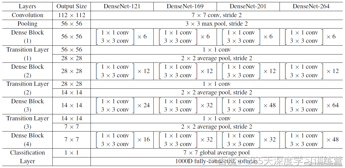表1 ImageNet数据集上所采用的DenseNet结构

4、与其他算法效果对比

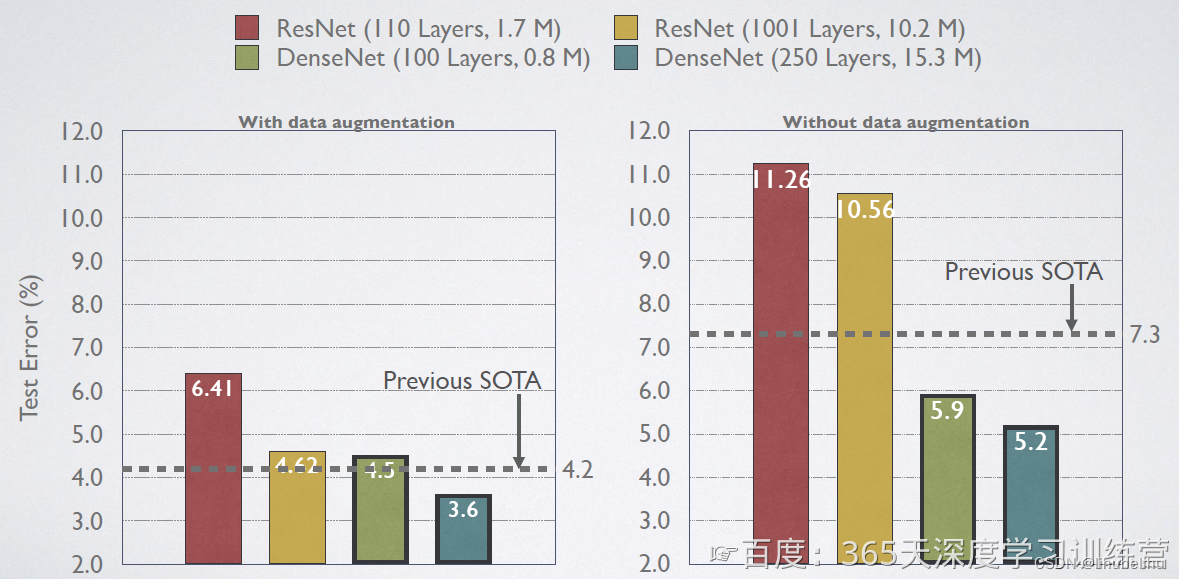在CIFAR-100数据集上ResNet vs DenseNet

5、使用Pytorch实现DenseNet121

这里我们采用Pytorch框架来实现DenseNet，首先实现DenseBlock中的内部结构，这里是BN+ReLU+1x1Conv+BN+ReLU+3x3Conv结构，最后也加入dropout层以用于训练过程

二、用pytorch具体代码实现DenseNet121

import torch
import torch.nn as nn
import torchvision.transforms as transforms
import torchvision
from torchvision import transforms, datasets
import os,PIL,pathlib,warnings
import torch.nn.functional as F

warnings.filterwarnings("ignore") #忽略警告信息

# 设置CPU/GPU
device = torch.device("cuda" if torch.cuda.is_available() else "cpu")

train_transforms = transforms.Compose([
transforms.Resize([224,224]),
transforms.ToTensor(),
transforms.Normalize(
mean = [0.485,0.456,0.406],
std = [0.229,0.224,0.225]
)
])

test_transforms = transforms.Compose([
transforms.Resize([224,224]),
transforms.ToTensor(),
transforms.Normalize(
mean = [0.485,0.456,0.406],
std = [0.229,0.224,0.225]
)
])

# 导入数据，与J1的数据是一样的
data_dir='./J3/bird_photos/'
data_dir=pathlib.Path(data_dir)

data_paths=list(data_dir.glob('*'))
classNames=[str(path).split('\\')[2] for path in data_paths]

num_classes=len(classNames)

total_data = datasets.ImageFolder(data_dir,transform = train_transforms)
total_data

代码输出：

Dataset ImageFolder
    Number of datapoints: 565
    Root location: J3\bird_photos
    StandardTransform
Transform: Compose(
               Resize(size=[224, 224], interpolation=bilinear, max_size=None, antialias=True)
               ToTensor()
               Normalize(mean=[0.485, 0.456, 0.406], std=[0.229, 0.224, 0.225])
           )

划分数据集
train_size = int(0.8 * len(total_data))
test_size = len(total_data) - train_size
train_dataset, test_dataset = torch.utils.data.random_split(total_data, [train_size, test_size])
print(train_dataset)
print(test_dataset)

batch_size = 8

train_dl = torch.utils.data.DataLoader(train_dataset,
batch_size=batch_size,
shuffle=True,
#num_workers=1
)
test_dl = torch.utils.data.DataLoader(test_dataset,
batch_size=batch_size,
shuffle=True,
#num_workers=1
)

for X, y in test_dl:
print("Shape of X [N, C, H, W]: ", X.shape)
print("Shape of y: ", y.shape, y.dtype)
break

for X, y in train_dl:
print("Shape of X [N, C, H, W]: ", X.shape)
print("Shape of y: ", y.shape, y.dtype)
break

from collections import OrderedDict
import torch
import torch.nn as nn
import torch.nn.functional as F

# BN+ReLU+1x1Conv+BN+ReLU+3x3Conv结构，最后也加入dropout层以用于训练过程
class _DenseLayer(nn.Sequential):
'''Basic unit of DenseBlock (using bottleneck layer)'''
def __init__(self,num_input_features,growth_rate,bn_size,drop_rate):
super(_DenseLayer,self).__init__()
self.add_module('norm1',nn.BatchNorm2d(num_input_features))
self.add_module('relu1',nn.ReLU(inplace=True))
self.add_module('conv1',nn.Conv2d(num_input_features, bn_size*growth_rate,kernel_size=1,stride=1,bias=False))

self.add_module('norm2',nn.BatchNorm2d(bn_size*growth_rate))
self.add_module('relu2',nn.ReLU(inplace=True))
self.add_module('conv2',nn.Conv2d(bn_size*growth_rate,growth_rate,kernel_size=3,stride=1,padding=1,bias=False))

self.drop_rate = drop_rate

def forward(self,x):
new_features =super(_DenseLayer,self).forward(x)
if self.drop_rate>0:
new_features = F.dropout(new_features,p=self.drop_rate,training=self.training)
return torch.cat([x,new_features],1)

# DenseBlock模块
# 内部是密集连接方式（输入特征数线性增长）

class _DenseBlock(nn.Sequential):
def __init__(self,num_layers,num_input_features,bn_size,growth_rate,drop_rate):
super(_DenseBlock,self).__init__()
for i in range(num_layers):
layer = _DenseLayer(
num_input_features+i*growth_rate,
growth_rate,
bn_size,
drop_rate
)
self.add_module('denselayer%d'%(i+1,),layer)

# Transition模块
# 实现Transition层，主要是一个卷积层和一个池化层
'''Transition layer between two adjacent DenseBlock'''
class _Transition(nn.Sequential):
def __init__(self,num_input_feature,num_output_features):
super(_Transition,self).__init__()
self.add_module('norm',nn.BatchNorm2d(num_input_feature))
self.add_module('relu',nn.ReLU(inplace=True))
self.add_module('conv',nn.Conv2d(
num_input_feature,
num_output_features,
kernel_size=1,
stride=1,
bias=False
))
self.add_module('pool',nn.AvgPool2d(2,stride=2))

# 实现DenseNet网络
# DenseNet-BC model
class DenseNet(nn.Module):
def __init__(self,growth_rate=32,block_config=(6,12,24,16),num_init_features=64,bn_size=4,
compression_rate=0.5,drop_rate=0,num_classes=1000):
"""
:param growth_rate:(int) number of filters used in DenseLayer.'k' in the paper
:param block_config:(list of 4 ints) number of layers in eatch DenseBlock
:param num_init_features:(int) number of filters in the first Conv2d
:param bn_size:(int) the factor using in the bottleneck layer
:param compression_rate: (float) the compression rate used in Transition Layer
:param drop_rate:(float) the drop rate after each DenseLayer
:param num_classes:(int) number of classes for classification
"""
super(DenseNet,self).__init__()
# first Conv2d
self.features =nn.Sequential(OrderedDict([
('conv0',nn.Conv2d(3,num_init_features,kernel_size=7,stride=2,padding=3,bias=False)),
('norm0',nn.BatchNorm2d(num_init_features)),
('relu0',nn.ReLU(inplace=True)),
('pool0',nn.MaxPool2d(3,stride=2,padding=1))
]))

# DenseBlock
num_features =num_init_features
for i,num_layers in enumerate(block_config):
block=_DenseBlock(
num_layers,
num_features,
bn_size,
growth_rate,
drop_rate
)
self.features.add_module('denseblock%d'%(i+1),block)
num_features += num_layers*growth_rate
if i != len(block_config)-1:
transition = _Transition(
num_features,
int(num_features*compression_rate
))
self.features.add_module('transition%d'%(i+1),transition)
num_features =int(num_features*compression_rate)


# final bn+ReLU
self.features.add_module('norm5',nn.BatchNorm2d(num_features))
self.features.add_module('relu5',nn.ReLU(inplace=True))

#分类层
#classification layer
self.classifier =nn.Linear(num_features,num_classes)

#参数初始化
#params initialization
for m in self.modules():
if isinstance(m,nn.Conv2d):
nn.init.kaiming_normal_(m.weight)
elif isinstance(m,nn.BatchNorm2d):
nn.init.constant(m.bias,0)
nn.init.constant(m.weight,1)
elif isinstance(m,nn.Linear):
nn.init.constant_(m.bias,0)

def forward(self,x):
features=self.features(x)
out=F.avg_pool2d(features,7,stride=1).view(features.size(0),-1)
out=self.classifier(out)
return out

# 选择不同网络参数，就可以实现不同深度的DenseNet，这里实现DenseNet-121网络，而且Pytorch提供了预训练好的网络参数
def densenet121(pretrained=False,**kwargs):
"""DenseNet121"""
model = DenseNet(num_init_features=64,growth_rate=32,block_config=(6,12,24,16),**kwargs)

if pretrained:
#'.'s are no longer allowed in module names, but pervious DenseLayer
# has keys 'norm.1','relu.1','conv.1','norm.2','relu.2','conv.2'
# They are also in the checkpoints in model_urls. This pattern is used
# to find such keys.
pattern =re.compile(
r'^(.*denselayer\d+\.(?:norm|relu|conv))\.((?:[12])\.(?:weight|bias|running_mean|running_var))$')
state_dict = model_zoo.load_url(model_urls['densenet121'])
for key in list(state_dict.keys()):
res = pattern.match(key)
if res:
new_key= res.group(1)+ res.group(2)
state_dict[new_key]= state_dict[key]
del state_dict[key]
model.load_state_dict(state_dict)
return model

model=densenet121().to(device)

# 统计模型参数量以及其他指标
import torchsummary as summary
summary.summary(model,(3,224,224))

# 编写训练函数
def train(dataloader,model,loss_fn,optimizer):
size = len(dataloader.dataset)
num_batches = len(dataloader)

train_acc,train_loss = 0,0

for X,y in dataloader:
X,y = X.to(device),y.to(device)

pred = model(X)
loss = loss_fn(pred,y)

optimizer.zero_grad()
loss.backward()
optimizer.step()

train_loss += loss.item()
train_acc += (pred.argmax(1) == y).type(torch.float).sum().item()

train_loss /= num_batches
train_acc /= size

return train_acc,train_loss

# 编写测试函数
def test(dataloader, model, loss_fn):
size = len(dataloader.dataset) # 测试集的大小
num_batches = len(dataloader) # 批次数目, (size/batch_size，向上取整)
test_loss, test_acc = 0, 0

# 当不进行训练时，停止梯度更新，节省计算内存消耗
with torch.no_grad():
for imgs, target in dataloader:
imgs, target = imgs.to(device), target.to(device)

# 计算loss
target_pred = model(imgs)
loss = loss_fn(target_pred, target)

test_loss += loss.item()
test_acc += (target_pred.argmax(1) == target).type(torch.float).sum().item()

test_acc /= size
test_loss /= num_batches

return test_acc, test_loss

import copy

loss_fn = nn.CrossEntropyLoss()
learn_rate = 1e-4
# SGD与Adam优化器，选择其中一个
# opt = torch.optim.SGD(model.parameters(),lr=learn_rate)
opt = torch.optim.Adam(model.parameters(),lr=learn_rate)

scheduler=torch.optim.lr_scheduler.StepLR(opt,step_size=1,gamma=0.9) #定义学习率高度器

epochs = 100 #设置训练模型的最大轮数为100，但可能到不了100
patience=10 #早停的耐心值，即如果模型连续10个周期没有准确率提升，则跳出训练

train_loss=[]
train_acc=[]
test_loss=[]
test_acc=[]
best_acc = 0 #设置一个最佳的准确率，作为最佳模型的判别指标
no_improve_epoch=0 #用于跟踪准确率是否提升的计数器
epoch=0 #用于统计最终的训练模型的轮数，这里设置初始值为0；为绘图作准备，这里的绘图范围不是epochs = 100

#开始训练
for epoch in range(epochs):

model.train()
epoch_train_acc,epoch_train_loss = train(train_dl,model,loss_fn,opt)

model.eval()
epoch_test_acc,epoch_test_loss = test(test_dl,model,loss_fn)



if epoch_test_acc > best_acc:
best_acc = epoch_test_acc
best_model = copy.deepcopy(model)



no_improve_epoch=0 #重置计数器
#保存最佳模型的检查点
PATH='./J3_best_model(121).pth'
torch.save({
'epoch':epoch,
'model_state_dict':best_model.state_dict(),
'optimizer_state_dict':opt.state_dict(),
'loss':epoch_test_loss,
},PATH)
else:
no_improve_epoch += 1


if no_improve_epoch >= patience:
print(f"Early stoping triggered at epoch {epoch+1}")
break #早停

train_acc.append(epoch_train_acc)
train_loss.append(epoch_train_loss)
test_acc.append(epoch_test_acc)
test_loss.append(epoch_test_loss)

scheduler.step() #更新学习率

lr = opt.state_dict()['param_groups'][0]['lr']

template = ('Epoch:{:2d}, Train_acc:{:.1f}%, Train_loss:{:.3f}, Test_acc:{:.1f}%, Test_loss:{:.3f}, Lr:{:.2E}')
print(template.format(epoch+1, epoch_train_acc*100, epoch_train_loss,epoch_test_acc*100, epoch_test_loss, lr))

# 保存最佳模型到文件中
PATH='./j3_best_model_121.pth' #保存的参数文件名
torch.save(model.state_dict(),PATH)

print('Done')
print(epoch)
print('no_improve_epoch:',no_improve_epoch)

代码输出：

Epoch: 1, Train_acc:54.0%, Train_loss:4.302, Test_acc:66.4%, Test_loss:1.682, Lr:9.00E-05
Epoch: 2, Train_acc:75.7%, Train_loss:1.219, Test_acc:77.9%, Test_loss:0.824, Lr:8.10E-05
Epoch: 3, Train_acc:80.5%, Train_loss:0.662, Test_acc:77.0%, Test_loss:0.747, Lr:7.29E-05
Epoch: 4, Train_acc:85.4%, Train_loss:0.475, Test_acc:82.3%, Test_loss:0.610, Lr:6.56E-05
Epoch: 5, Train_acc:89.6%, Train_loss:0.375, Test_acc:81.4%, Test_loss:0.546, Lr:5.90E-05
Epoch: 6, Train_acc:89.8%, Train_loss:0.343, Test_acc:87.6%, Test_loss:0.456, Lr:5.31E-05
Epoch: 7, Train_acc:91.6%, Train_loss:0.318, Test_acc:88.5%, Test_loss:0.395, Lr:4.78E-05
Epoch: 8, Train_acc:93.1%, Train_loss:0.241, Test_acc:85.8%, Test_loss:0.373, Lr:4.30E-05
Epoch: 9, Train_acc:92.7%, Train_loss:0.254, Test_acc:89.4%, Test_loss:0.403, Lr:3.87E-05
Epoch:10, Train_acc:94.0%, Train_loss:0.203, Test_acc:87.6%, Test_loss:0.305, Lr:3.49E-05
Epoch:11, Train_acc:95.6%, Train_loss:0.152, Test_acc:87.6%, Test_loss:0.319, Lr:3.14E-05
Epoch:12, Train_acc:97.8%, Train_loss:0.133, Test_acc:90.3%, Test_loss:0.529, Lr:2.82E-05
Epoch:13, Train_acc:94.2%, Train_loss:0.177, Test_acc:87.6%, Test_loss:0.425, Lr:2.54E-05
Epoch:14, Train_acc:97.8%, Train_loss:0.143, Test_acc:86.7%, Test_loss:0.339, Lr:2.29E-05
Epoch:15, Train_acc:97.1%, Train_loss:0.135, Test_acc:90.3%, Test_loss:0.354, Lr:2.06E-05
Epoch:16, Train_acc:98.5%, Train_loss:0.099, Test_acc:92.0%, Test_loss:0.335, Lr:1.85E-05
Epoch:17, Train_acc:97.3%, Train_loss:0.116, Test_acc:92.9%, Test_loss:0.262, Lr:1.67E-05
Epoch:18, Train_acc:98.9%, Train_loss:0.084, Test_acc:91.2%, Test_loss:0.290, Lr:1.50E-05
Epoch:19, Train_acc:98.2%, Train_loss:0.100, Test_acc:91.2%, Test_loss:0.317, Lr:1.35E-05
Epoch:20, Train_acc:97.8%, Train_loss:0.132, Test_acc:91.2%, Test_loss:0.310, Lr:1.22E-05
Epoch:21, Train_acc:97.6%, Train_loss:0.114, Test_acc:90.3%, Test_loss:0.339, Lr:1.09E-05
Epoch:22, Train_acc:98.7%, Train_loss:0.095, Test_acc:91.2%, Test_loss:0.287, Lr:9.85E-06
Epoch:23, Train_acc:98.0%, Train_loss:0.087, Test_acc:90.3%, Test_loss:0.277, Lr:8.86E-06
Epoch:24, Train_acc:98.0%, Train_loss:0.114, Test_acc:92.0%, Test_loss:0.285, Lr:7.98E-06
Epoch:25, Train_acc:97.3%, Train_loss:0.113, Test_acc:92.0%, Test_loss:0.291, Lr:7.18E-06
Epoch:26, Train_acc:99.3%, Train_loss:0.058, Test_acc:92.0%, Test_loss:0.317, Lr:6.46E-06
Early stoping triggered at epoch 27
Done
26
no_improve_epoch: 10

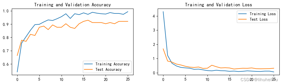
# 结果可视化
# Loss与Accuracy图

import matplotlib.pyplot as plt
#隐藏警告
import warnings
warnings.filterwarnings("ignore") #忽略警告信息
plt.rcParams['font.sans-serif'] = ['SimHei'] # 用来正常显示中文标签
plt.rcParams['axes.unicode_minus'] = False # 用来正常显示负号
plt.rcParams['figure.dpi'] = 100 #分辨率

epochs_range = range(epoch)

plt.figure(figsize=(12, 3))
plt.subplot(1, 2, 1)

plt.plot(epochs_range, train_acc, label='Training Accuracy')
plt.plot(epochs_range, test_acc, label='Test Accuracy')
plt.legend(loc='lower right')
plt.title('Training and Validation Accuracy')

plt.subplot(1, 2, 2)
plt.plot(epochs_range, train_loss, label='Training Loss')
plt.plot(epochs_range, test_loss, label='Test Loss')
plt.legend(loc='upper right')
plt.title('Training and Validation Loss')
plt.show()

代码输出：

预测：

from PIL import Image

classes = list(total_data.class_to_idx)

def predict_one_image(image_path, model, transform, classes):

test_img = Image.open(image_path).convert('RGB')
plt.imshow(test_img) # 展示预测的图片

test_img = transform(test_img)
img = test_img.to(device).unsqueeze(0)

model.eval()
output = model(img)

_,pred = torch.max(output,1)
pred_class = classes[pred]
print(f'预测结果是：{pred_class}')

import os
from pathlib import Path
import random
image=[]
def image_path(data_dir):
file_list=os.listdir(data_dir) #列出四个分类标签
data_file_dir=file_list #从四个分类标签中随机选择一个
data_dir=Path(data_dir)
for i in data_file_dir:
i=Path(i)
image_file_path=data_dir.joinpath(i) #拼接路径
data_file_paths=image_file_path.iterdir() #罗列文件夹的内容
data_file_paths=list(data_file_paths) #要转换为列表
image.append(data_file_paths)
file=random.choice(image) #从所有的图像中随机选择一类
file=random.choice(file) #从选择的类中随机选择一张图片
return file

data_dir='J3/bird_photos'
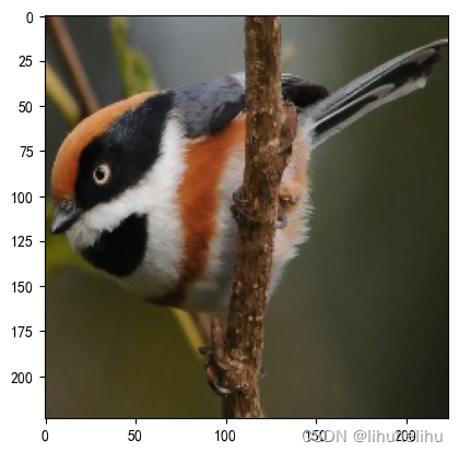
image_path=image_path(data_dir)

# 预测训练集中的某张照片
predict_one_image(image_path=image_path,
model=model,
transform=train_transforms,
classes=classes)

代码输出：

预测结果是：Black Throated Bushtiti

# 模型评估
# 将参数加载到model当中
best_model.load_state_dict(torch.load(PATH,map_location=device))
epoch_test_acc,epoch_test_loss=test(test_dl,best_model,loss_fn)
epoch_test_acc,epoch_test_loss

代码输出：

(0.9203539823008849, 0.28216510570297637)

三、总结

根据表1，可以实现DenseNet-169、DenseNet-201、DenseNet-264。在DenseNet-121的基础上，也就是在上面的代码中找到参数block_config=(6,12,24,16)，作出如下的修改：

DenseNet-169：block_config=(6,12,32,32)

DenseNet-201：block_config=(6,12,48,32)

DenseNet-264：block_config=(6,12,64,48)

四、DenseNet-121网络结构图