


文章目录
数据分析——Adventure项目分析
内容摘要
一、项目简介
- 公司业务简介
Adventure Works Cycle是国内一家制造公司,该公司生产和销售金属和复合材料自行车在全国各个市场。销售方式主要有两种,前期主要是分销商模式,但是2018年公司实现财政收入目标后,2019就开始通过公司自有网站获取线上商户进一步扩大市场。 - 分析背景
2019年12月业务组组长需要向领导汇报2019年11月自行车销售情况,为精细化运营提供数据支持,能精准的定位目标客户群体。 - 分析目的
1、如何制定销售策略,调整产品结构,才能保持高速增长,获取更多的收益,占领更多市场份额,是公司最关心的问题。
2、报告通过对整个公司的自行车销量持续监测和分析,掌握公司自行车销售状况、走势的变化,为客户制订、调整和检查销售策略,完善产品结构提供依据。 - 数据源及表内信息
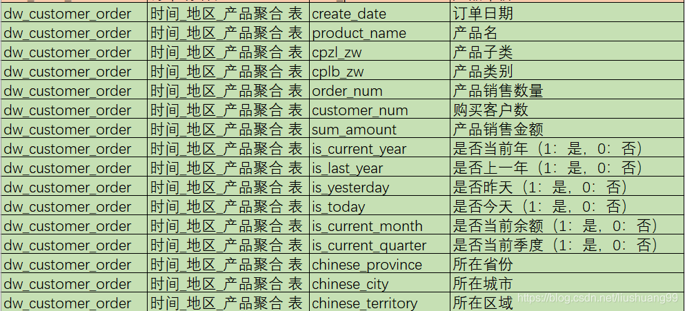
dw_customer_order 产品销售信息事实表
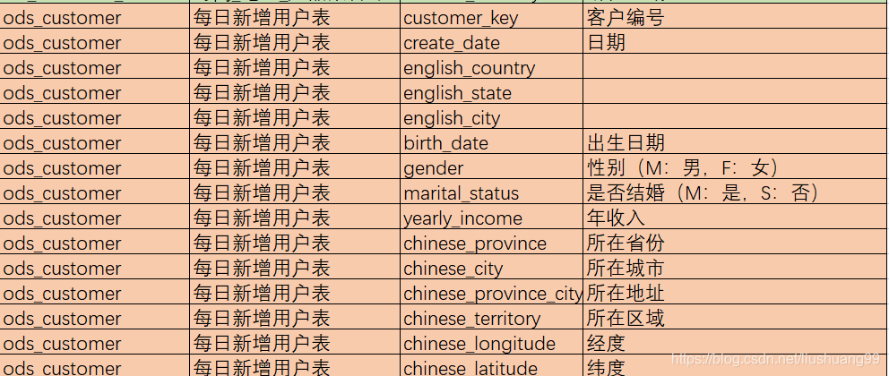
ods_customer 每天新增客户信息表
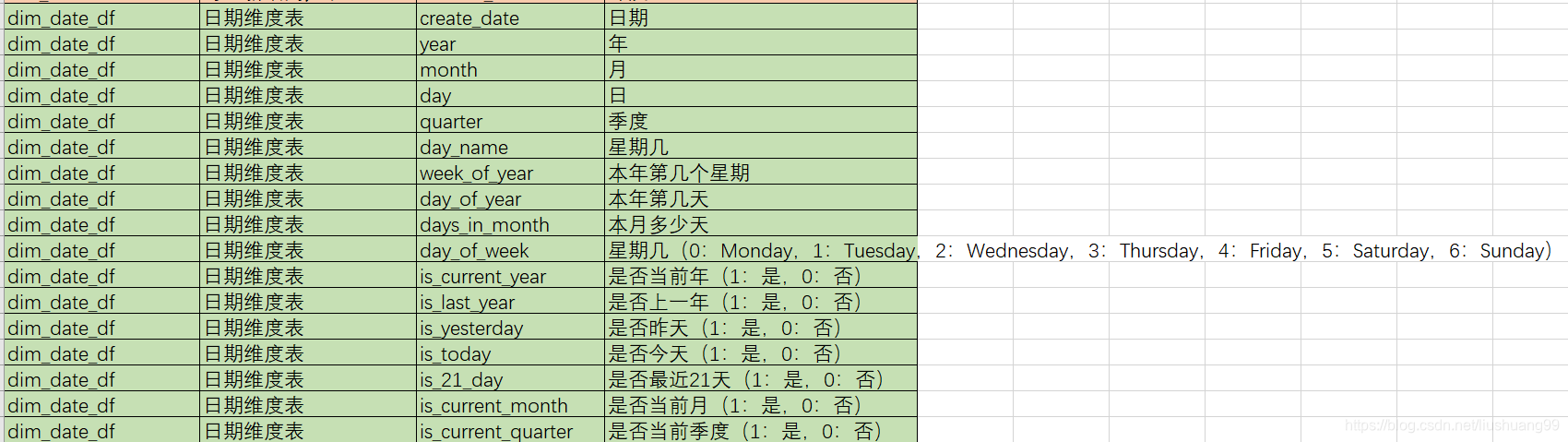
dim_date_df 日期表
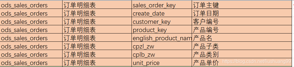
ods_sales_orders 订单明细表
二、分析思路
- 分析思路

三、分析过程
0、数据准备及清洗
(1) 导入模块
import pandas as pd
import numpy as np
import pymysql
pymysql.install_as_MySQLdb()
from sqlalchemy import create_engine
- 创建数据库引擎并读取数据库
engine = "mysql+pymysql://frogdata001:XXXXXXXXX/adventure?charset=gbk"
sql = "select * from dw_customer_order"
gather_customer_order=pd.read_sql_query(sql,con=engine)
(2) 简单了解数据
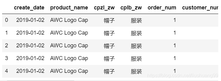
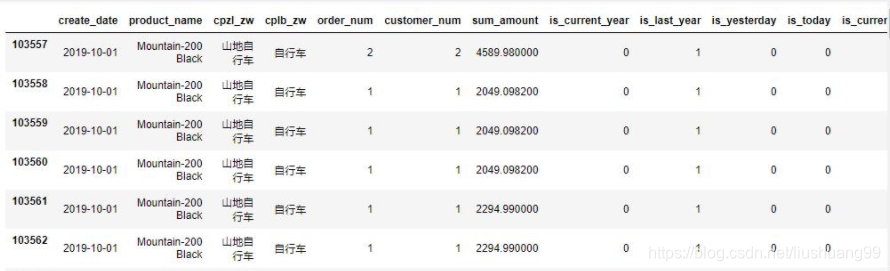
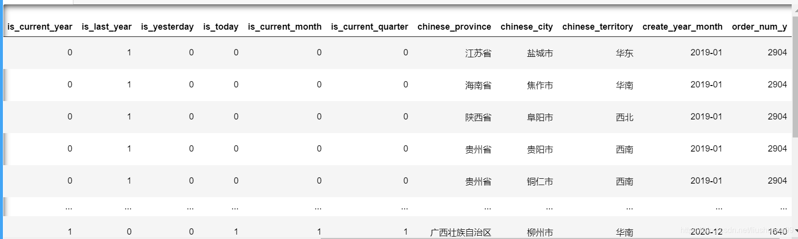
gather_customer_order.head()
gather_customer_order.info()

(3) 数据处理
可以看出create_date时间的格式不对,将其修改为datetime64的格式,并且为了后续计算方便将其年-月进行提取
#将本字段的格式修改成datetime64的形式
gather_customer_order['create_date'] = gather_customer_order['create_date'].astype('datetime64')
#增加create_year_month月份字段。按月维度分析时使用
#使用的是strftime函数,%M代表的是分钟,%m代表的是月份
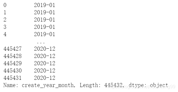
gather_customer_order['create_year_month'] = gather_customer_order['create_date'].apply(lambda x:x.strftime("%Y-%m"))
#查看数据
gather_customer_order['create_year_month']
- 筛选数据
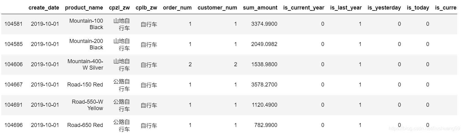
从cplb_zw筛选出自行车的数据用作分析
#筛选产品类别为自行车的数据
#需要用准确定位即.loc来索引
#!需要注意的是loc后面需要用中括号,不能用小括号!
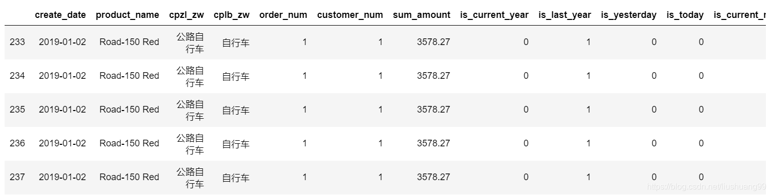
gather_customer_order = gather_customer_order.loc[gather_customer_order['cplb_zw']=='自行车']
gather_customer_order.head()

1、整体销售表现
- 对整体销售表现分析
- 其时间维度:月份;
- 表现字段:销售量、销售金额
(1) 自行车整体销售量表现
#利用groupby聚合月份,对order_num、sum_amount求和
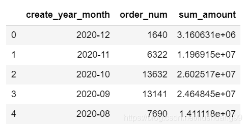
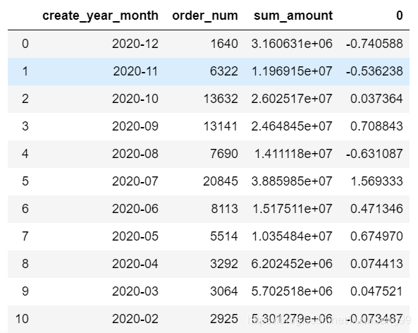
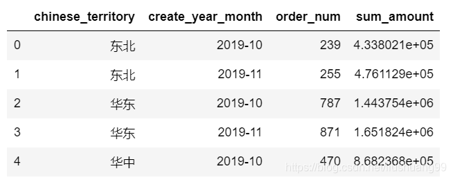
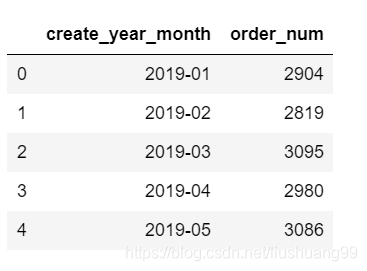
overall_sales_performance = gather_customer_order.groupby("create_year_month").agg({"order_num":"sum","sum_amount":"sum"}).sort_values("create_year_month",ascending=False).reset_index()
#按日期降序排序,方便计算环比
overall_sales_performance.head()
- 利用diff函数求环比。
- diff函数是前一个数-后一个数,之后再除以前一个数,结果作为环比
#求每月自行车销售订单量环比,观察最近一年数据变化趋势
#环比是本月与上月的对比,例如本期2019-02月销售额与上一期2019-01月销售额做对比
#计算公式是(本月-上月)/上月
#使用diff函数第一行是Nan,因此正好diff只除以其所对应的原始数据即可,但是要注意乘以负号
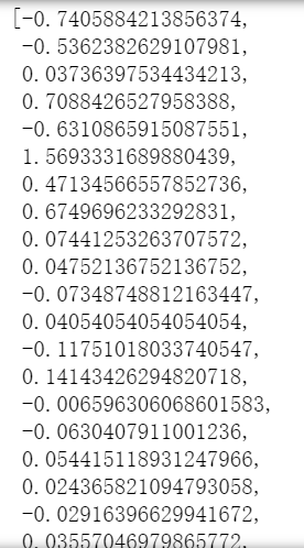
order_num_diff = list((overall_sales_performance.order_num.diff()/overall_sales_performance.order_num)*(-1))
order_num_diff.pop(0) #删除列表中第一个元素,第一个元素是nan
order_num_diff.append(0) #将0新增到列表末尾
order_num_diff
- 将计算好的环比拼接在overall_sales_performance 数据集中,暂时先不命名,等后续销售金额环比算完后统一修改
#将环比转化为DataFrame
#pd.DataFrame就可以转换成
#利用pd.concat进行拼接的时候一定要注意:axis是行拼接!
overall_sales_performance = pd.concat([overall_sales_performance,pd.DataFrame(order_num_diff)],axis=1)
(2) 自行车整体销售金额表现
- 操作过程跟自行车整体销量相同,前期数据集已经准备好,直接对销售金额进行环比计算即可
#求每月自行车销售金额环比
sum_amount_diff = list((overall_sales_performance["sum_amount"].diff()/overall_sales_performance["sum_amount"])*(-1))
sum_amount_diff.pop(0) #删除列表中第一个元素
sum_amount_diff.append(0) #将0新增到列表末尾
sum_amount_diff
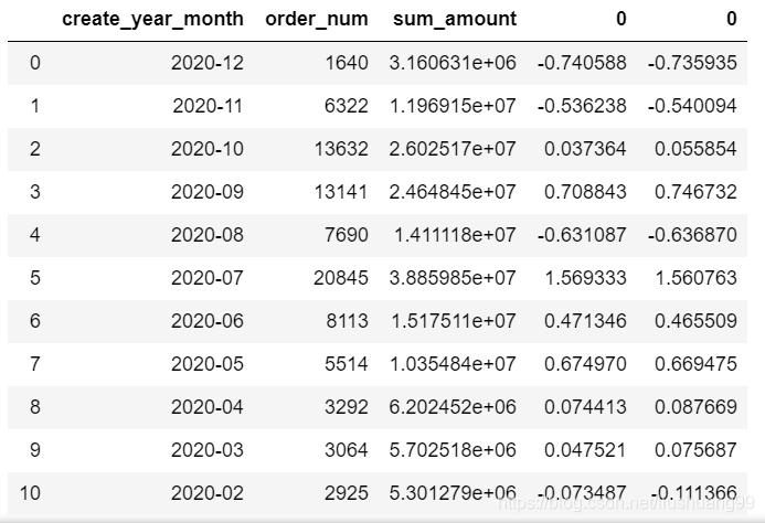
#将环比转化为DataFrame
overall_sales_performance = pd.concat([overall_sales_performance,pd.DataFrame(sum_amount_diff)],axis=1)
overall_sales_performance
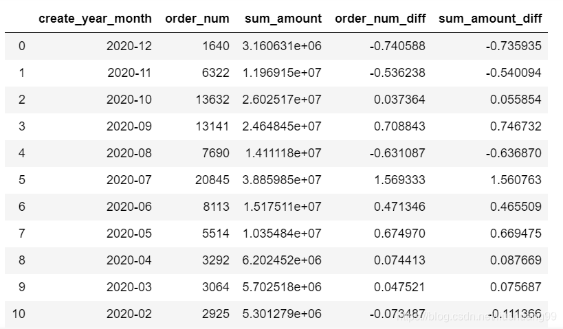
- 对销量和销售金额的环比进行重命名
销量环比:order_num_diff
销售金额环比:sum_amount_diff
#修改一下列名
overall_sales_performance.columns=['create_year_month','order_num','sum_amount','order_num_diff','sum_amount_diff']
overall_sales_performance
- 随后将整理好的overall_sales_performance数据存入数据库,为PowerBI绘制提供数据基础
#将数据存入数据库
engine = create_engine("mysql+pymysql://XXXXXXXXXXXXXXXX:3306/XXXXXXX?charset=gbk")
overall_sales_performance.to_sql('pt_overall_sale_performance',con=engine,if_exists="append")
(3) 可视化展示
-
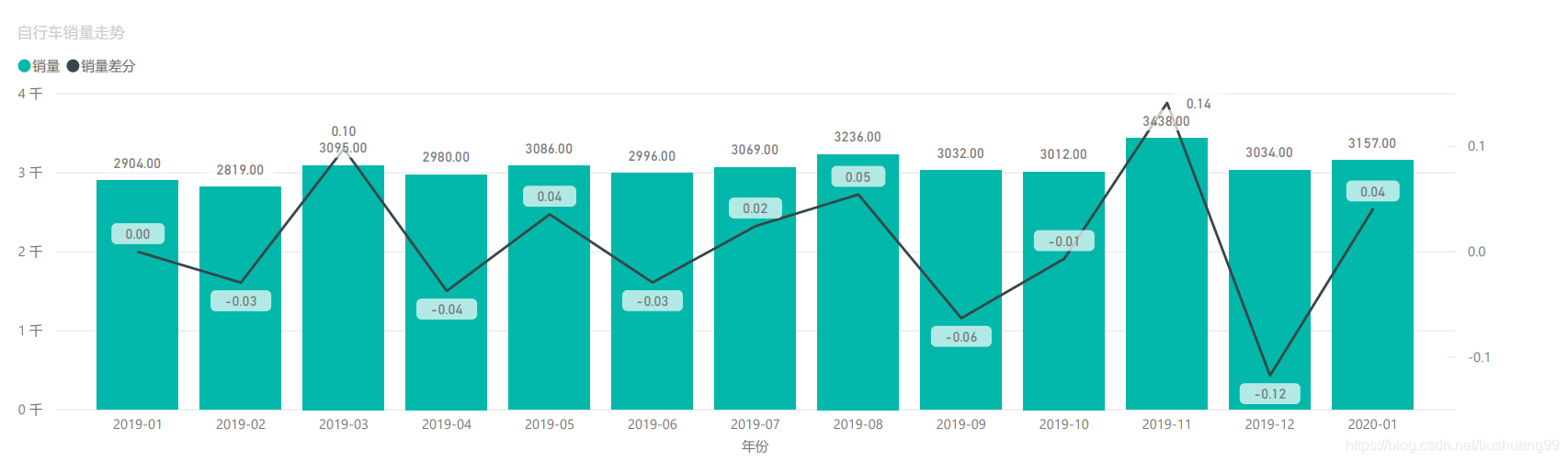
自行车销量走势情况
-
根据图可以看出:
- (1)2019年11月自行车销量最高,为3438辆;
- (2)2019年11月自行车销量环比增量最高,为0.14;
- (3)自行车销量在3000辆上下波动,普遍波动程度在10个点以内。
-
自行车销售金额走势情况
-
根据图可以看出:
- (1)2019年11月自行车销售金额最高,为660万;
- (2)2019年11月自行车销售金额环比增量最高,为0.18;
- (3)自行车销售金额在600万上下波动,普遍波动程度在10个点以内。

-
2019年11月自行车的销售程度明显增加,销量和销售金额都有明显大幅度的提高
2、地域销售表现
(1) 2019年11月地区销售表现
- 针对不同地区的销售情况进行分析
- 数据清洗及筛选
- 筛选出2019年10月、11月的销售数据
- 分析不同地区的11月销售情况
- 分析不同地区的11月销售环比情况
#筛选2019年10、11月的自行车数据
gather_customer_order_10_11 = gather_customer_order.loc[(gather_customer_order["create_year_month"]=="2019-10")
                                                        |(gather_customer_order["create_year_month"]=="2019-11")]
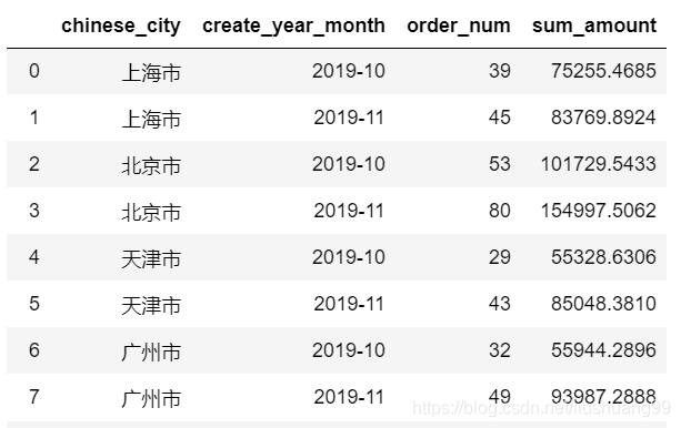
- 数据分组:依旧根据月份进行分组,对销量和销售金额进行求和
#按照区域、月分组,订单量求和,销售金额求和
gather_customer_order_10_11_group= gather_customer_order_10_11.groupby(['chinese_territory','create_year_month']).agg({
    'order_num':'sum','sum_amount':'sum'}).reset_index()
-
环比计算:利用pct_change()函数
-
本次环比计算的难点:需要对不同的地区进行环比计算
-
计算逻辑:
- (1)先将不同地区分开
- (2)遍历不同地区的数据,利用pct_change()求其环比
- (3)将环比数据拼接起来,转换成Series格式拼接在原来的数据集上面
#将区域存为列表
region_list= gather_customer_order_10_11_group["chinese_territory"].unique()
#查看具体区域名称
region_list
#array(['东北', '华东', '华中', '华北', '华南', '台港澳', '西北', '西南'], dtype=object)
#pct_change()当前元素与先前元素的相差百分比,求不同区域10月11月环比
#先准备好Series和列表
order_x = pd.Series([])
amount_x = pd.Series([])
#遍历不同地区,提取其10、11月的销量、销售金额数据,再进行环比计算
for i in region_list:
a=gather_customer_order_10_11_group.loc[gather_customer_order_10_11_group['chinese_territory']==i]['order_num'].pct_change(1)
b=gather_customer_order_10_11_group.loc[gather_customer_order_10_11_group['chinese_territory']==i]['sum_amount'].pct_change(1)
order_x=order_x.append(a)
amount_x = amount_x.append(b)
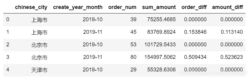
#将计算好的环比数据拼接在数据集后面
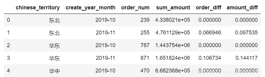
gather_customer_order_10_11_group['order_diff']=order_x
gather_customer_order_10_11_group['amount_diff']=amount_x
# 需要注意的是,每一组数据的第一行的数据都是NaN,需要将NaN值进行填充
gather_customer_order_10_11_group = gather_customer_order_10_11_group.fillna(0)
#10月11月各个区域自行车销售数量、销售金额环比
gather_customer_order_10_11_group.head()
- 将数据保存在数据库中
#将数据存入数据库
engine = "mysql+pymysql://XXXXXXXXX/XXXXXXXX?charset=gbk"
gather_custXXXXXXXXomer_order_10_11_group.to_sql('pt_bicy_november_territory',con=engine,if_exists="append")
(2) 2019年11月TOP10销量城市环比
-
数据清洗与筛选
- 从上一次操作中的数据集中提取11月的数据
#筛选11月自行车交易数据
gather_customer_order_11 = gather_customer_order_10_11.loc[gather_customer_order_10_11["create_year_month"]=="2019-11"]
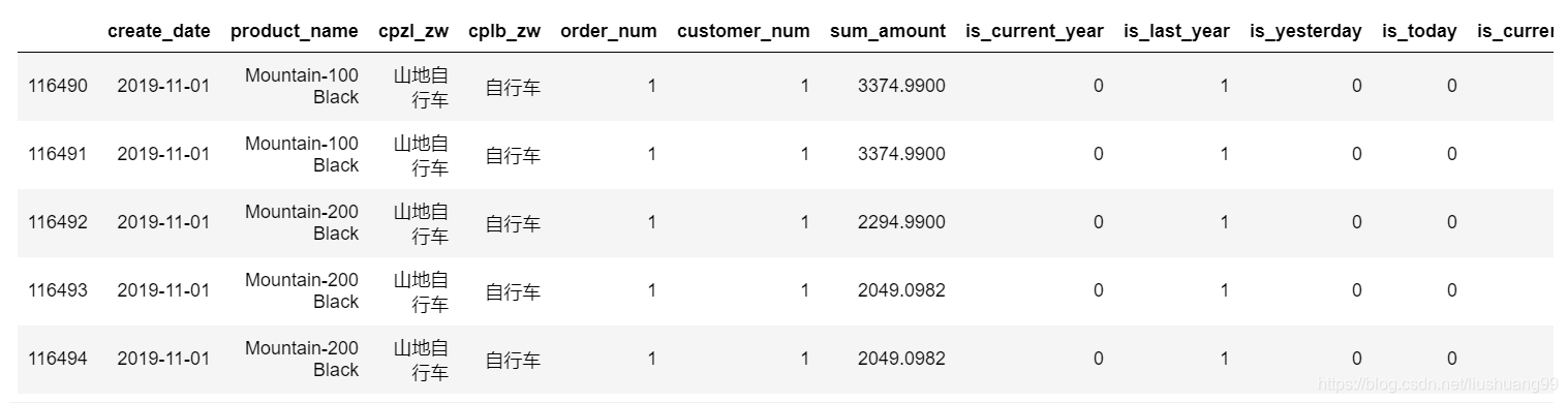
#查看数据
gather_customer_order_11.head()
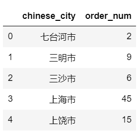
- 数据分组:根据chinese_city城市分组,对销售量进行求和统计
gather_customer_order_city_11= gather_customer_order_11.groupby("chinese_city").agg({"order_num":"sum"}).reset_index()
gather_customer_order_city_11.head()
- 数据筛选:挑选出11月销量TOP10的城市名称
#11月自行车销售数量前十城市,导出数据集为gather_customer_order_city_head
gather_customer_order_city_head = gather_customer_order_city_11.sort_values('order_num',ascending=False).head(10)
#查看TOP10城市名称
gather_customer_order_city_head['chinese_city'].values
#array(['北京市', '广州市', '深圳市', '上海市', '郑州市', '天津市', '重庆市', '武汉市', '长沙市','西安市'], dtype=object)
-
数据再筛选
- 根据已知的11月销量TOP10的城市名称,从2019年10月、11月的数据集中,提取销量和销售金额数据(利用isin()函数)
- 数据再分组:按照TOP10城市的名称进行分组
- 分析2019年11月销量TOP10城市的环比(利用pct_change()函数)
#数据再筛选
#利用isin函数从10月11月自行车销售数据中,筛选出2019年11月销售前十城市
gather_customer_order_10_11_head = gather_customer_order_10_11.loc[gather_customer_order_10_11["chinese_city"].isin(gather_customer_order_city_head['chinese_city'].values)]
#数据再分组
#分组计算前十城市,自行车销售数量销售金额
gather_customer_order_city_10_11 = gather_customer_order_10_11_head.groupby(['chinese_city','create_year_month']).agg(
    {'order_num':'sum','sum_amount':'sum'}).reset_index()
#TOP10城市环比计算
#TOP10城市的名称
city_top_list = gather_customer_order_city_10_11['chinese_city'].unique()
#准备Series和列表
order_top_x = pd.Series([])
amount_top_x = pd.Series([])
#遍历TOP10城市,提取其对应的销量、销售金额,利用pct_change()函数进行环比
for i in city_top_list:
    #print(i)
    a= gather_customer_order_city_10_11[gather_customer_order_city_10_11['chinese_city']==i]['order_num'].pct_change(1)
    b= gather_customer_order_city_10_11[gather_customer_order_city_10_11['chinese_city']==i]['sum_amount'].pct_change(1)
    order_top_x = order_top_x.append(a)
    amount_top_x = amount_top_x.append(b)
 #将环比数据拼接在数据集后面
 #order_diff销售数量环比,amount_diff销售金额环比
gather_customer_order_city_10_11['order_diff']=order_top_x
gather_customer_order_city_10_11['amount_diff']=amount_top_x
#NaN值替换
gather_customer_order_city_10_11 = gather_customer_order_city_10_11.fillna(0)
(3) 可视化展示
-
区域销量环比增速图
-
根据图可以看出:
- (1)自行车销售共分:华东、华中、西南、华北、华南、西北、东北和台港澳8个区域;
- (2)2019年10月-11月,华东地区自行车销量最高,分别为:787台和871台;
- (3)台港澳区域因数据量少其环比呈现较高水平,但在分析时应考虑具体销量,避免出现辛普森悖论;
- (4)除台港澳区域外,西北地区销量环比增速最快,为0.28。

-
TOP10城市销量环比增速情况
-
根据图可以看出:
- (1)2019年11月自行车销量TOP10城市分别为:北京、上海、广州、重庆、深圳、武汉、天津、长沙、郑州和西安;
- (2)2019年10月-11月,北京市自行车销量最高,分别为:53台和80台;
- (3)郑州市销量环比增速最大,达到了1.00。

3、产品销售表现
(1) 细分市场销量表现
- 数据筛选
- 细分市场是指自行车的类别:公路、山地和旅游
- 仍以时间(月份)为尺度进行分析,因此需要对时间进行分组
#利用gather_customer_order数据表对时间进行分组
#求每个月自行车累计销售数量
gather_customer_order_group_month = gather_customer_order.groupby('create_year_month').agg({'order_num':'sum'}).reset_index()
- 数据处理
- 将每月的总销量(gather_customer_order_group_month)与订单信息(gather_customer_order)进行拼接
- 计算每一个订单在当月的占比(自行车销量/自行车每月销量占比),为之后按照细分市场聚合做准备
#合并自行车销售信息表+自行车每月累计销售数量表,pd.merge
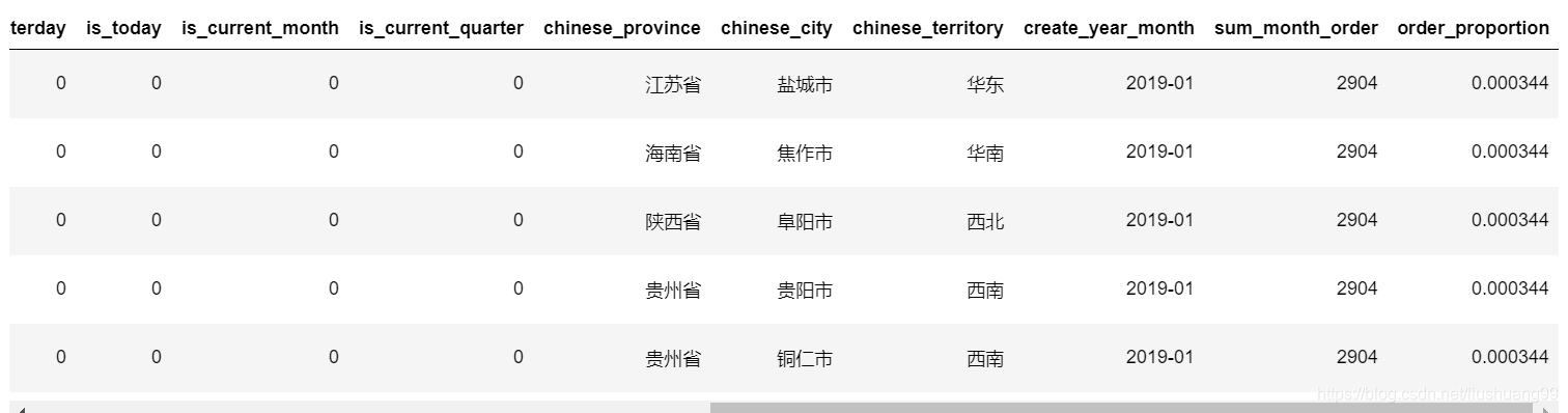
order_num_proportion = pd.merge(gather_customer_order,gather_customer_order_group_month,how='left',on='create_year_month')
#计算自行车销量/自行车每月销量占比x,及订单占当月的比例
order_num_proportion['order_proportion'] = order_num_proportion['order_num_x']/order_num_proportion['order_num_y']
#重命名sum_month_order:自行车每月销售量
order_num_proportion = order_num_proportion.rename(columns={'order_num_y':'sum_month_order'})
#查看自行车有那些产品子类
gather_customer_order['cpzl_zw'].unique()
#array(['山地自行车', '公路自行车', '旅游自行车'], dtype=object)
#将每月自行车销售信息存入数据库
engine = 'mysql+pymysql://XXXXXXXX/XXXXXXXX?charset=gbk'
order_num_proportion.to_sql('pt_bicycle_product_sales_month_4',con=engine,if_exists='replace')
(2) 公路自行车销量表现
- 数据筛选及处理
- 筛选出公路自行车的数据
- 时间维度:月份;信息维度:不同型号公路自行车
- 对月份和型号进行分组统计(gather_customer_order_road_month)
#数据筛选,挑选出公路自行车的数据
gather_customer_order_road = gather_customer_order[gather_customer_order['cpzl_zw'] == '公路自行车']
#对日期和不同型号进行分组
#求公路自行车不同型号产品销售数量
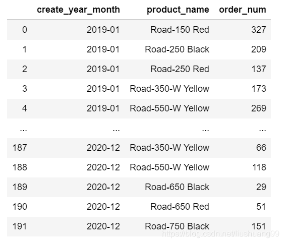
gather_customer_order_road_month = gather_customer_order_road.groupby(by = ['create_year_month','product_name']).agg(
{'order_num':'sum'}).reset_index()
#添加自行车子类标签
gather_customer_order_road_month['cpzl_zw'] = '公路自行车'
-
数据整合
- 需要整理对应类型每月的销量情况(gather_customer_order_road_month_sum)
- 将每月的销量情况与不同类别销量情况进行整合
- 计算占比情况
#每个月公路自行车累计销售数量
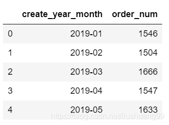
gather_customer_order_road_month_sum = gather_customer_order_road_month.groupby('create_year_month').agg({'order_num':'sum'}).reset_index()
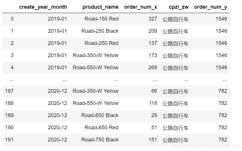
#合并公路自行车gather_customer_order_road_month与每月累计销售数量
#用于计算不同型号产品的占比
gather_customer_order_road_month = pd.merge(gather_customer_order_road_month,gather_customer_order_road_month_sum,
                                            how='left',on='create_year_month')
(3) 山地自行车销量表现
-
数据处理过程与公路自行车相同
-
主要流程:
- (1)筛选对应的自行车子类;
- (2)对日期和型号进行分组,计算订单数量
- (3)对当前自行车子类按月份进行分组,统计订单数量
- (4)数据拼接,将两组数据集进行拼接
# 筛选
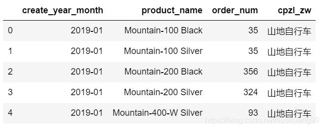
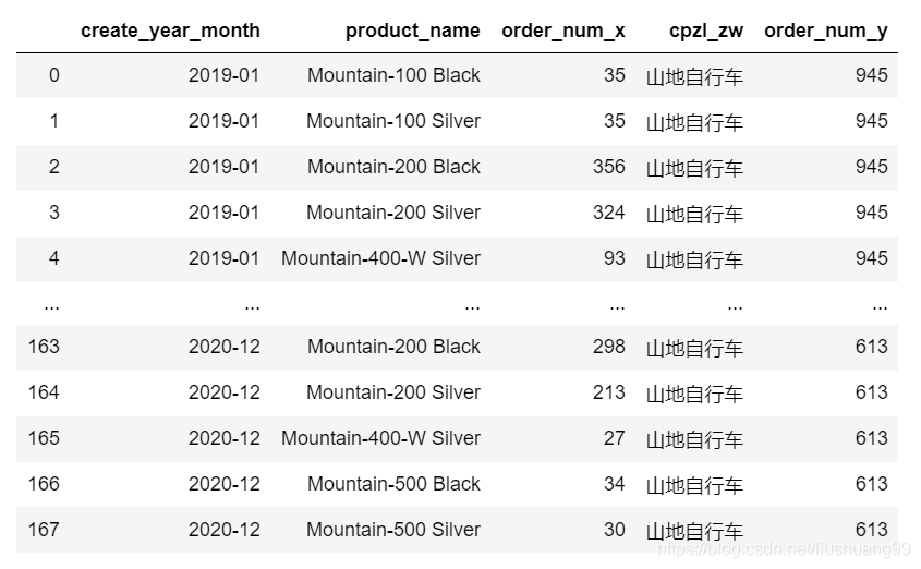
gather_customer_order_Mountain = gather_customer_order[gather_customer_order['cpzl_zw'] == '山地自行车']
#求山地自行车不同型号产品销售数量
gather_customer_order_Mountain_month = gather_customer_order_Mountain.groupby(['create_year_month','product_name']).agg(
{'order_num':'sum'}).reset_index()
#添加自行车子类标签
gather_customer_order_Mountain_month['cpzl_zw'] = '山地自行车'
#每个月山地自行车累计销售数量
gather_customer_order_Mountain_month_sum = gather_customer_order_Mountain_month.groupby('create_year_month').agg({'order_num':'sum'}).reset_index()
#gather_customer_order_Mountain_month_sum.head()

#合并山地自行车hz_customer_order_Mountain_month与每月累计销售数量
#用于计算不同型号产品的占比
gather_customer_order_Mountain_month = pd.merge(gather_customer_order_Mountain_month,gather_customer_order_Mountain_month_sum,
                                                how='left',on='create_year_month')
(4) 旅游自行车销量表现
-
数据处理过程与公路自行车相同
-
主要流程:
- (1)筛选对应的自行车子类;
- (2)对日期和型号进行分组,计算订单数量
- (3)对当前自行车子类按月份进行分组,统计订单数量
- (4)数据拼接,将两组数据集进行拼接
#数据筛选
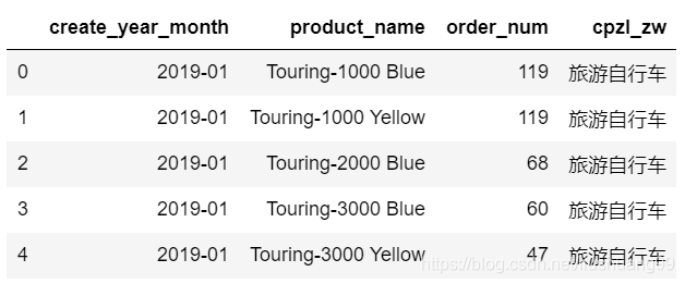
gather_customer_order_tour = gather_customer_order[gather_customer_order['cpzl_zw'] == '旅游自行车']
#求旅游自行车不同型号产品销售数量
gather_customer_order_tour_month = gather_customer_order_tour.groupby(['create_year_month','product_name']).agg(
{'order_num':'sum'}).reset_index()
#添加子类标签
gather_customer_order_tour_month['cpzl_zw'] = '旅游自行车'
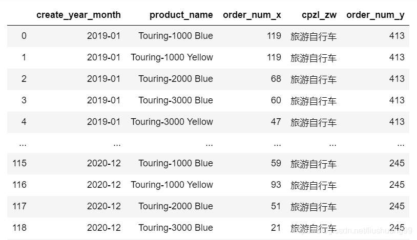
#每个月旅游自行车销量统计
gather_customer_order_tour_month_sum = gather_customer_order_tour_month.groupby('create_year_month').agg({'order_num':'sum'}).reset_index()
#gather_customer_order_tour_month_sum.head() 查看
gather_customer_order_tour_month = pd.merge(gather_customer_order_tour_month,gather_customer_order_tour_month_sum,how='left',on='create_year_month')
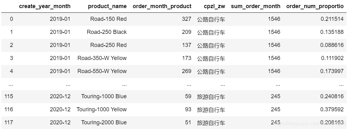
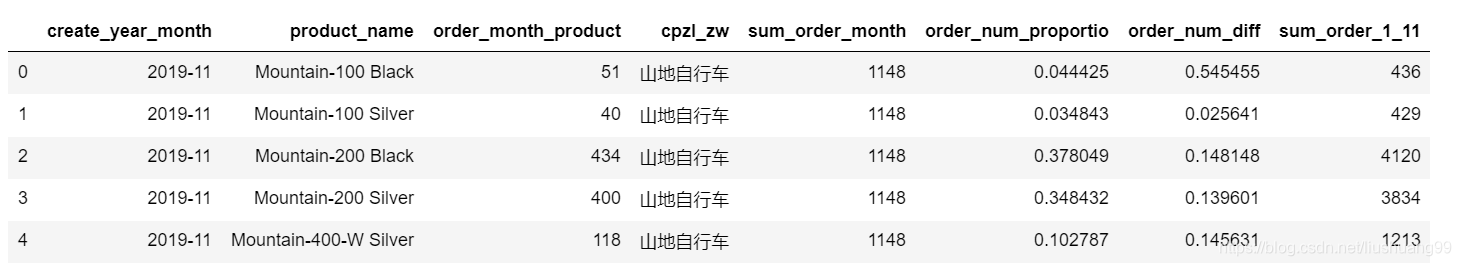
(5) 自行车子类数据整合
- 将自行车子类数据进行整合,并计算每月每型号自行车占比情况
#将山地自行车、旅游自行车、公路自行车每月销量信息合并
gather_customer_order_month = pd.concat([gather_customer_order_road_month,gather_customer_order_Mountain_month,
gather_customer_order_tour_month])
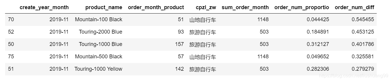
#各类自行车,销售量占每月自行车总销售量比率
gather_customer_order_month['order_num_proportio'] = gather_customer_order_month.apply(lambda x:x[2]/x[4],axis=1)
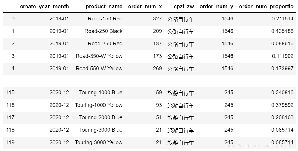
#整理列标签信息
#order_month_product当月产品累计销量
#sum_order_month当月自行车总销量
gather_customer_order_month.rename(columns={'order_num_x':'order_month_product','order_num_y':'sum_order_month'},inplace=True)
#保存数据到数据库
#将数据存入数据库
engine = 'mysql+pymysql://XXXXXXX/XXXXXXX?charset=gbk'
gather_customer_order_month.to_sql('pt_bicycle_product_sales_order_month_4_DOUBLEYOOO',con=engine,if_exists='append')
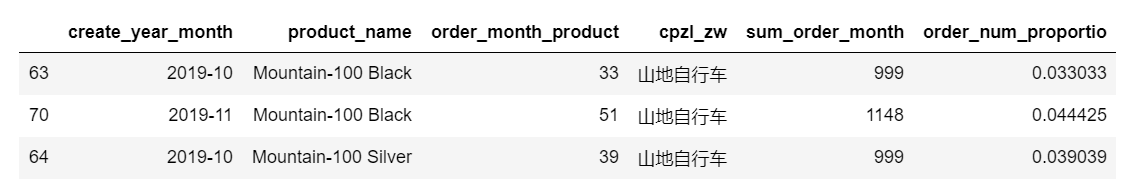
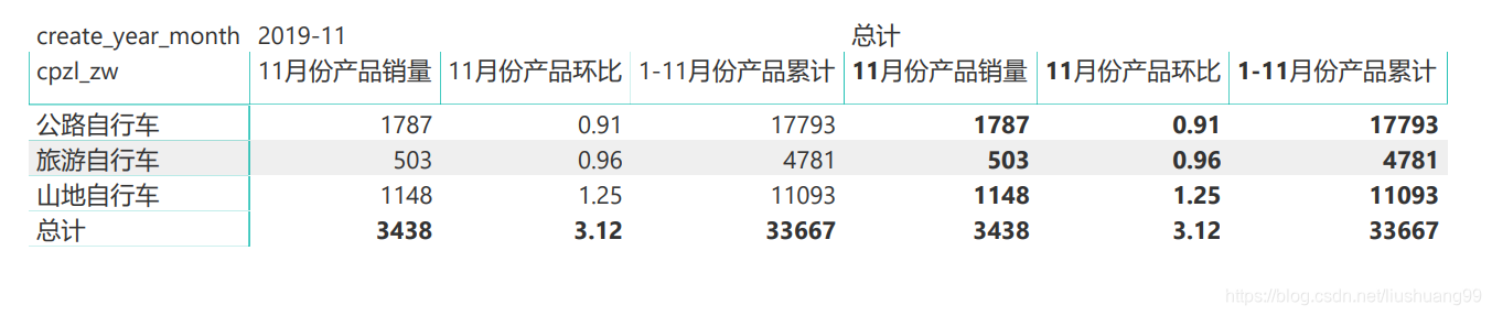
(6) 2019年11月自行车产品环比情况
- 数据筛选
-
筛选出2019年10月和11月的数据,并按照时间进行排序
-
跟之前求环比一样操作
- 先获取数据列表
- 遍历数据,找到销量进行环比计算(pct_change()函数)
- 拼接到数据集中,去除NaN值
-
#计算11月环比,先筛选10月11月数据
gather_customer_order_month_10_11 = gather_customer_order_month[gather_customer_order_month.create_year_month.isin(['2019-10','2019-11'])]
#排序。将10月11月自行车销售信息排序
gather_customer_order_month_10_11 = gather_customer_order_month_10_11.sort_values(by = ['product_name','create_year_month'])
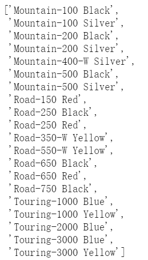
#查看具体名称
product_name  = list(gather_customer_order_month_10_11.product_name.drop_duplicates())
#计算自行车销售数量环比
order_top_x = pd.Series([])
for i in product_name:
    order_top = gather_customer_order_month_10_11[gather_customer_order_month_10_11['product_name']==i]['order_month_product'].pct_change(1)
    order_top_x = order_top_x.append(order_top)
#拼接
gather_customer_order_month_10_11['order_num_diff'] = order_top_x
#填充NaN值
gather_customer_order_month_10_11['order_num_diff'].fillna(0,inplace=True)
#筛选出11月自行车数据
gather_customer_order_month_11 = gather_customer_order_month_10_11[gather_customer_order_month_10_11['create_year_month'] == '2019-11']

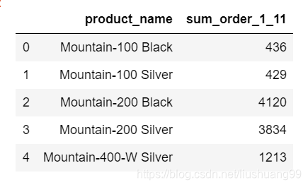
(7) 计算2019年1月-11月自行车产品累计销量
- 数据筛选
#筛选2019年1月至11月自行车数据,这里使用的是‘~’取对立面
#isin里面不能时str格式
gather_customer_order_month_1_11 = gather_customer_order_month[~gather_customer_order_month.create_year_month.isin(
    ['2019-12','2020-12','2020-11','2020-10','2020-09','2020-08','2020-07','2020-06','2020-05','2020-04','2020-03','2020-02','2020-01'])]
#计算2019年1月至11月自行车累计销量
gather_customer_order_month_1_11_sum = gather_customer_order_month_1_11.groupby(by = 'product_name').order_month_product.sum().reset_index()
#重命名sum_order_1_11:1-11月产品累计销量
gather_customer_order_month_1_11_sum = gather_customer_order_month_1_11_sum.rename(columns = {'order_month_product':'sum_order_1_11'})
(8) 关联自行车销量、环比和累计销量
累计销量我们在gather_customer_order_month_1_11_sum中已计算好,11月自行车环比、及产品销量占比在gather_customer_order_month_11已计算好,这里我们只需将两张表关联起来,用pd.merge()
#按相同字段product_name产品名,合并两张表
gather_customer_order_month_11 = pd.merge(gather_customer_order_month_11,gather_customer_order_month_1_11_sum,how='left',on='product_name')
#存入数据库
engine = 'mysql+pymysql://XXXXXXX/XXXXXX?charset=gbk'
gather_customer_order_month_11.to_sql('pt_bicycle_product_sales_order_month_11_DOUBLEYOOO',con=engine,if_exists='append')
(9) 可视化展示
-
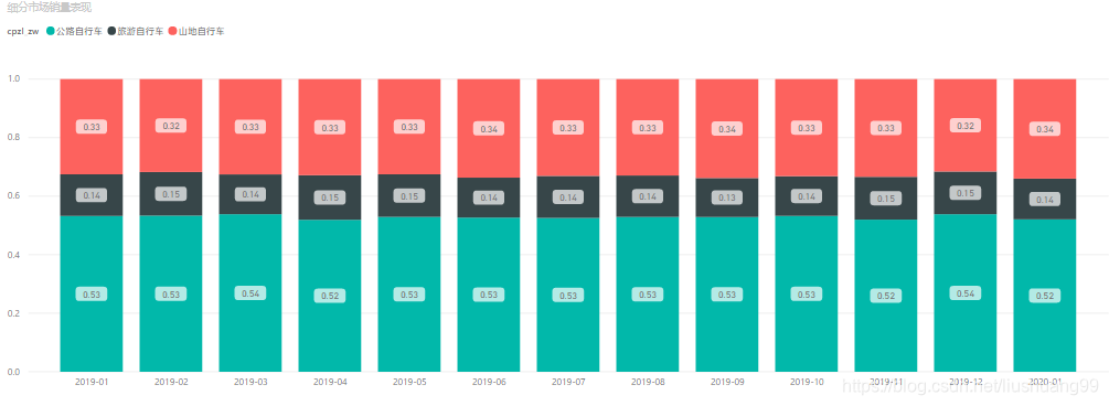
细分市场销量表现
-
根据图可以看出:
- (1)三个自行车类型中销量占比情况为:公路自行车>山地自行车>旅游自行车;
- (2)公路自行车每月的销量占比均超过50%;
- (3)三种自行车类型每月销量变化不大;
- (4)山地自行车11月销量环比最大为1.25
-
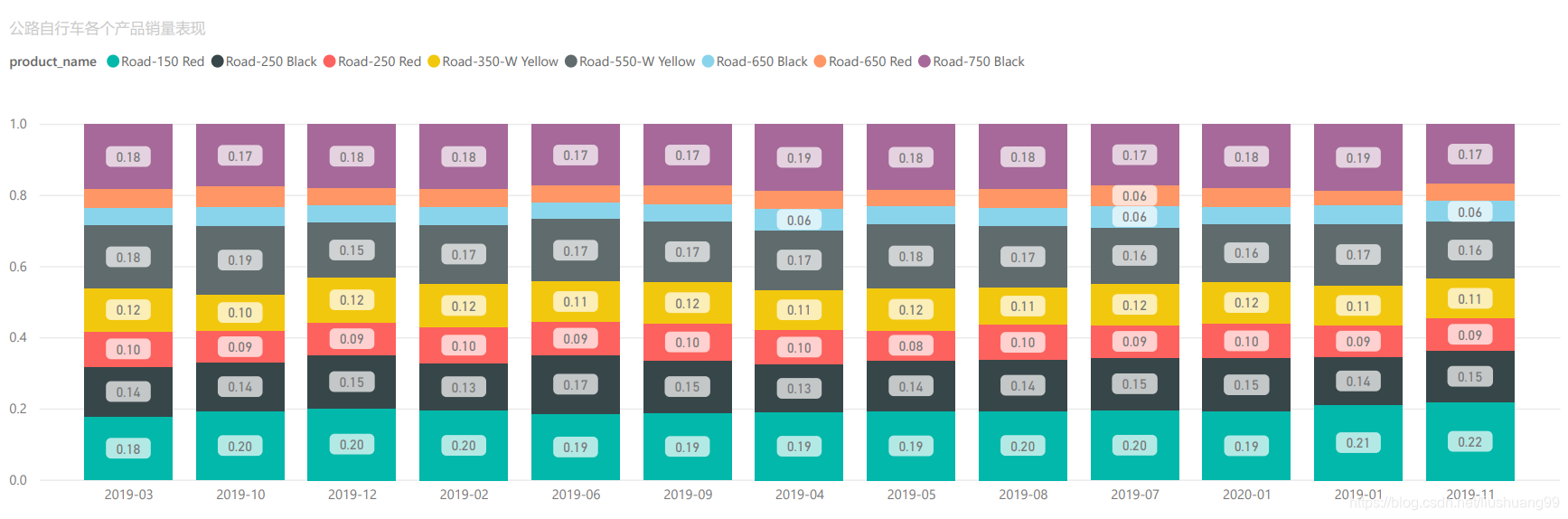
公路自行车各个产品销量表现
-
根据图可以看出:
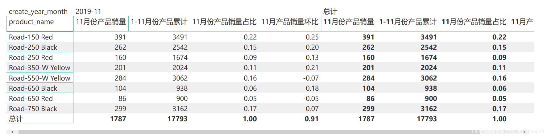
- (1)Road-150 Red每月销量都最高,均在18%以上;
- (2)Road-750 Black每月销量位列第二,均在17%以上;
- (3)Road-550-W Yellow每月销量位列第三,均在15%以上;
- (4)以上三个产品占公路自行车月销量的50%以上;
- (5)Road-150 Red 1-11月累计销量、11月销量、销量环比最高,分别为3491台、391台和25%;
- (6)Road-550-W Yellow和Road-650 Red 2019年11月销量出现负增长,其余都为正增长
-
旅游自行车各个产品销量表现
-
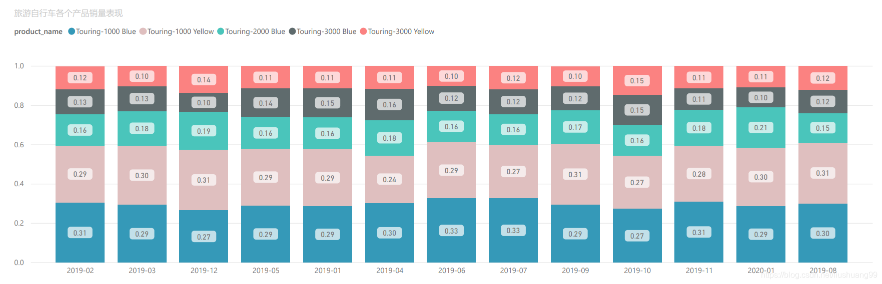
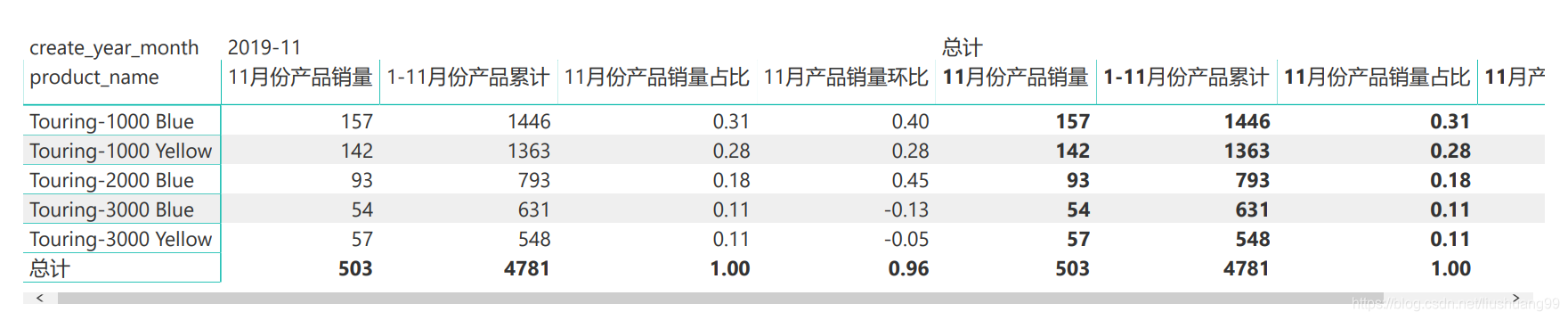
根据图可以看出:
- (1)Touring-1000 Blue每月销量都最高,均在27%以上;
- (2)Touring-1000 Yellow每月销量位列第二,均在24%以上;
- (3)以上两个产品占公路自行车月销量的51%以上;
- (4)Touring-1000 Blue 1-11月累计销量、11月销量、销量环比最高,分别为1446台、157台和31%;
- (5)Touring-3000 Blue和Touring-3000 Yellow 2019年11月销量出现负增长,其余都为正增长
-
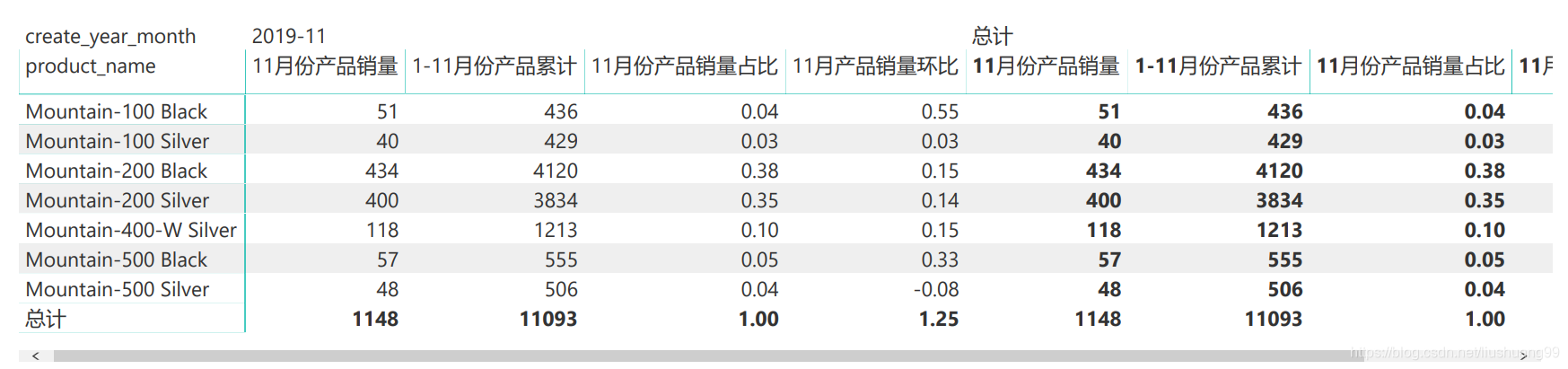
山地自行车各个产品销量表现
-
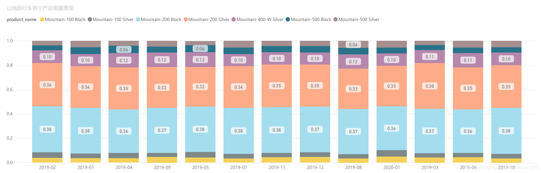
根据图可以看出:
- (1)Mountain-200 Black每月销量都最高,均在36%以上;
- (2)Mountain-200 Silver每月销量位列第二,均在33%以上;
- (3)以上两个产品占公路自行车月销量的69%以上;
- (4)Mountain-200 Black 1-11月累计销量、11月销量、销量环比最高,分别为4120台、434台和38%;
- (5)Mountain-500 Silver 2019年11月销量出现负增长,其余都为正增长
4、用户行为分析
- 用户行为分析主要对用户的年龄和性别进行分析
(1) 数据整理
-
数据筛选
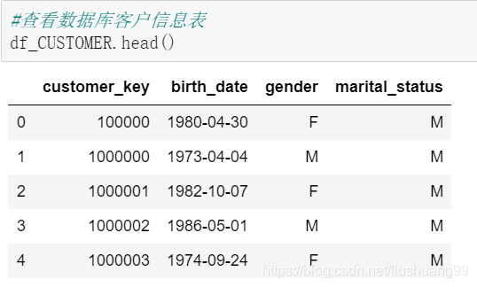
- 这里我们需要使用订单明细表:ods_sales_orders,ods_customer用户表
#读取数据库客户信息表
engine = create_engine('mysql://XXXXXX/XXXX?charset=gbk')
datafrog=engine
df_CUSTOMER = pd.read_sql_query("select customer_key,birth_date,gender,marital_status from ods_customer where create_date < '2019-12-1'",con = datafrog)
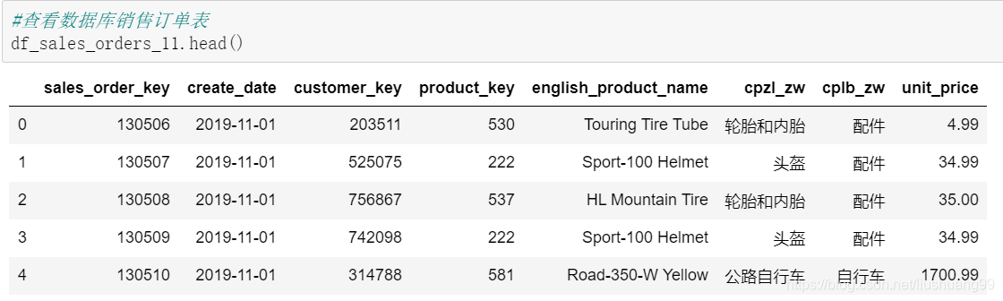
#读取数据库销售订单表
engine = create_engine('mysql://XXXX/XXX?charset=gbk')
datafrog=engine
df_sales_orders_11 = pd.read_sql_query("select * from ods_sales_orders where create_date>='2019-11-1' and create_date<'2019-12-1'",con = datafrog)
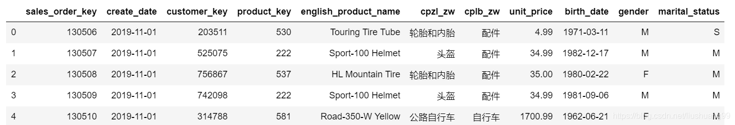
-
数据合并
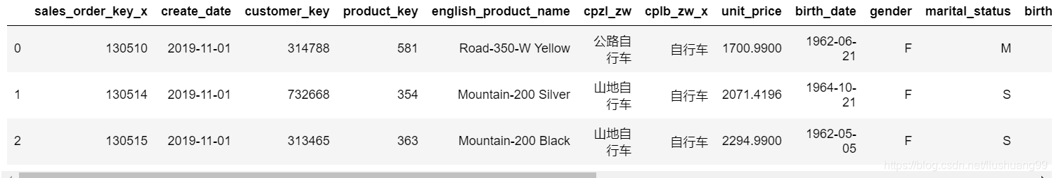
- 销售订单表中仅客户编号,无客户年龄性别等信息,需要将销售订单表和客户信息表合并
#pd.merge 合并
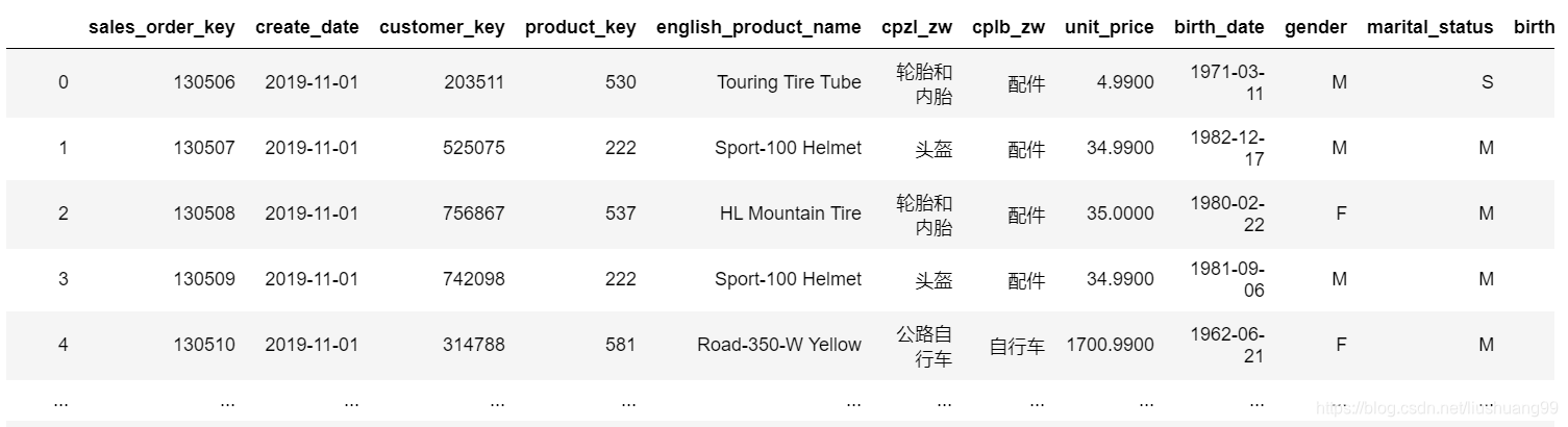
sales_customer_order_11=pd.merge(df_sales_orders_11,df_CUSTOMER,how='left',on='customer_key')
sales_customer_order_11.head()
-
数据清洗
- 将用户的birth_date只提取年份生成customer_birth_year保存
#将生日的年份提取出来
customer_birth_year = sales_customer_order_11['birth_date'].str.split('-',2).apply(lambda x :x[0] if type(x) == list else x)
customer_birth_year.name='birth_year'
#数据拼接,将年份拼接在数据集后面
sales_customer_order_11 = pd.concat([sales_customer_order_11,customer_birth_year],axis = 1)

(2) 用户年龄分析
- 首先计算年龄(2019年-出生年)
#修改出生年为int数据类型
sales_customer_order_11['birth_year'] = sales_customer_order_11['birth_year'].fillna(method='ffill').astype('int')
# 计算用户年龄
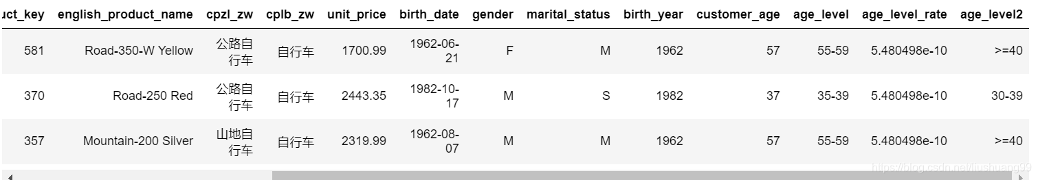
sales_customer_order_11['customer_age'] = 2019 - sales_customer_order_11['birth_year']
- 年龄分组(以5岁一档)
#年龄分层1
label = ['30-34','35-39','40-44','45-49','50-54','55-59','60-64']
number = [i for i in range(30 , 68 ,5)]
#新增'age_level'分层区间列
sales_customer_order_11['age_level'] = pd.cut(sales_customer_order_11['customer_age'],bins=number,labels=label) #right=True 表示右闭,False表示右开
- 筛选出自行车的数据
#筛选销售订单为自行车的订单信息
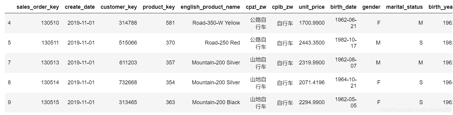
df_customer_order_bycle = sales_customer_order_11.loc[sales_customer_order_11['cplb_zw'] == '自行车']
# 计算年龄比率

##这个比率的意思是求单独每个用户的占总人数的占比,为下一步聚合提供准备
df_customer_order_bycle['age_level_rate'] = 1/(df_customer_order_bycle['customer_key'].sum())
- 年龄分层(按年岁分组)
#将年龄分为3个层次
df_customer_order_bycle['age_level2'] = pd.cut(df_customer_order_bycle['customer_age'],bins=[0,30,40,120],right=False,labels=['<=29','30-39','>=40'])
- 求每个年龄段购买量
# 求每个年龄段购买量
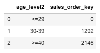
age_level2_count = df_customer_order_bycle.groupby(by = 'age_level2').sales_order_key.count().reset_index()
age_level2_count
- 将每个年龄段的消费订单与消费者的信息拼接
- 计算每一次消费的占比情况,为后续的分组整理做准备
#将每个年龄段的消费订单数与消费者信息结合
df_customer_order_bycle = pd.merge(df_customer_order_bycle,age_level2_count,on = 'age_level2').rename(columns = {'sales_order_key_y':'age_level2_count'})
#计算每一次消费的占比情况,后续的groupby做准备
df_customer_order_bycle['age_level2_rate'] = 1/df_customer_order_bycle['age_level2_count']
(3) 用户性别分析
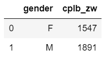
- 按照性别分组计算,计算不同性别的总人数
gender_count = df_customer_order_bycle.groupby(by = 'gender').cplb_zw.count().reset_index()
- 将性别分组与消费者情况相结合
- 计算每个消费者在当前性别中的比率
#将性别分组与消费者情况相结合
df_customer_order_bycle = pd.merge(df_customer_order_bycle,gender_count,on = 'gender').rename(columns = {'cplb_zw_y':'gender_count'})
df_customer_order_bycle['gender_rate'] = 1/df_customer_order_bycle['gender_count']
#df_customer_order_bycle 将11月自行车用户存入数据库
#存入数据库
engine = create_engine('mysql://XXXXXXX/XXXXX?charset=gbk')

datafrog=engine
df_customer_order_bycle.to_sql('pt_user_behavior_novembe',con = datafrog,if_exists='append', index=False)
(4) 可视化展示
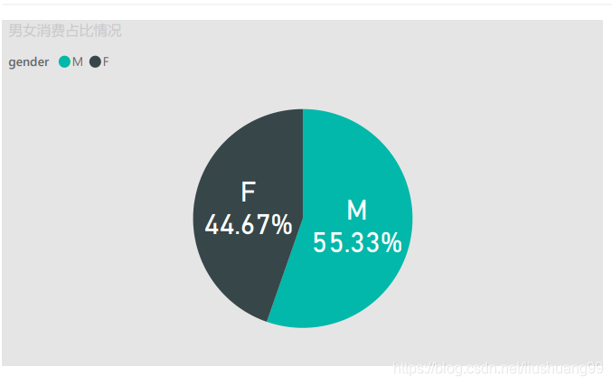
- 男女消费者消费占比情况
- 根据图可以看出:
- (1)男性消费者贡献主要的消费力,占55.33%;女性消费者消费占比为44.67%
- (1)男性消费者贡献主要的消费力,占55.33%;女性消费者消费占比为44.67%
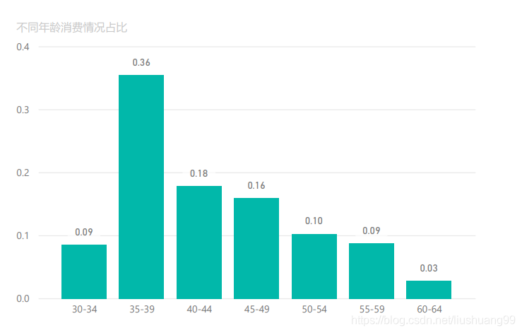
- 不同年龄消费情况占比
- 根据图可以看出:
- (1)消费者的年龄在30岁以上;
- (2)35-39岁的消费者占较大部分,约占36%;
- (3)随着年龄的增长消费力逐渐下降
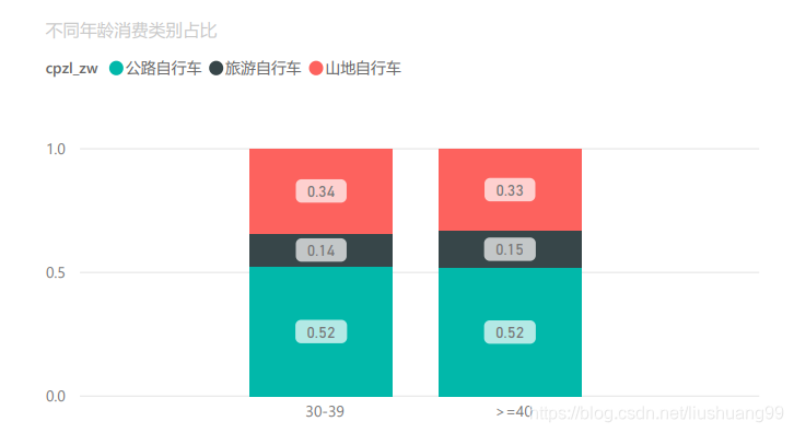
- 不同年龄具体消费情况占比
- 根据图可以看出:
- (1)两个年龄段中购买公路自行车占主要部分,约占52%,山地自行车次之,为33%;
- (2)两个年龄段相比之下,30-39岁消费者偏爱山地自行车,而40岁及以上的消费者多偏向与旅行自行车;
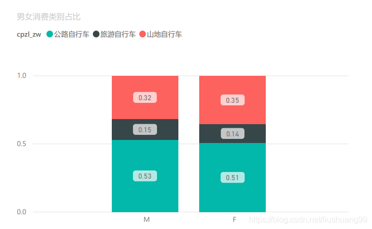
- 男女具体消费情况占比
- 根据图可以看出:
- (1)不同性别消费者的主要消费对象仍是公路自行车,占比均在50%以上;
- (2)男性消费者更偏爱公路自行车,女性消费者则偏爱山地自行车
5、热销产品分析
- 针对产品热度进行分析,主要分析销量热度和环比增速热度,限制范围为各热度的TOP10品牌
- 数据集:gather_customer_order
(1) 2019年11月销量TOP10品牌
-
数据筛选
- 筛选出2019年11月销量数据
#筛选11月数据
gather_customer_order_11 = gather_customer_order.loc[gather_customer_order['create_year_month'] == '2019-11']
-
数据处理
- 数据对不同品牌进行分组统计
- 对销量进行求和并进行降序排列
- 计算11月品牌环比(利用之前的数据集gather_customer_order_month_10_11,通过isin()函数进行提取)
#按照销量降序,取TOP10产品
customer_order_11_top10 = gather_customer_order_11.groupby(by = 'product_name').order_num.count().reset_index().\
                        sort_values(by = 'order_num',ascending = False).head(10)
#TOP10销量产品信息
list(customer_order_11_top10['product_name'])
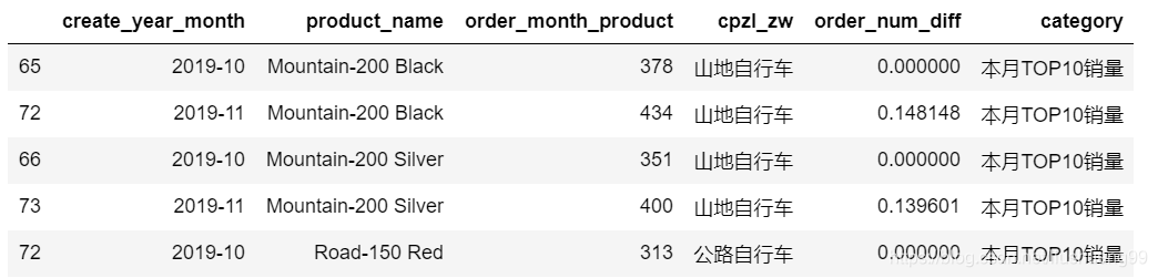
#提取gather_customer_order_month_10_11数据集的四个字段:create_year_month月份,product_name产品名,order_month_product本月销量,cpzl_zw产品类别,
order_num_diff本月产品销量环比
customer_order_month_10_11 = gather_customer_order_month_10_11[['create_year_month','product_name','order_month_product','cpzl_zw','order_num_diff']]
#把前十名的产品信息取出
customer_order_month_10_11 = customer_order_month_10_11[customer_order_month_10_11['product_name'].\
isin(list(customer_order_11_top10['product_name']))] #重命名
customer_order_month_10_11['category'] = '本月TOP10销量'
(2) 2019年11月增速TOP10品牌
-
数据筛选
- 利用gather_customer_order_month_10_11数据集,将2019年11月的数据筛选出来
- 按照环比数据进行降序排列
- 筛选出前10个品牌
customer_order_month_11 = gather_customer_order_month_10_11.loc[gather_customer_order_month_10_11['create_year_month'] == '2019-11'].\
                            sort_values(by = 'order_num_diff',ascending = False).head(10)
-
数据处理
- 从gather_customer_order_month_10_11数据集中提取增速TOP10的品牌数据,与上面TOP10销量数据拼接做准备
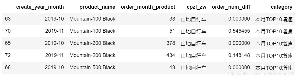
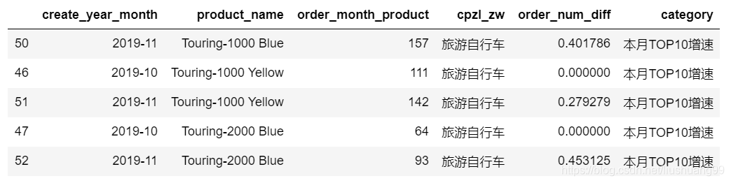
#找到增速最快的十个产品
customer_order_month_11_top10_seep = gather_customer_order_month_10_11.loc[gather_customer_order_month_10_11['product_name'].\
                                                        isin(list(customer_order_month_11['product_name']))]
#筛选出主要的四个字段:create_year_month月份,product_name产品名,order_month_product本月销量,cpzl_zw产品类别,
order_num_diff本月产品销量环比
customer_order_month_11_top10_seep = customer_order_month_11_top10_seep[['create_year_month','product_name','order_month_product','cpzl_zw','order_num_diff']]
#重命名
customer_order_month_11_top10_seep['category'] = '本月TOP10增速'
-
合并数据
- 将TOP10销量表和TOP10增速表拼接在一起
#axis = 0按照行维度合并,axis = 1按照列维度合并
hot_products_11 = pd.concat([customer_order_month_10_11,customer_order_month_11_top10_seep],axis = 0)
#存入数据库
engine = create_engine('mysql://XXXXXXX/XXXXXX?charset=gbk')
datafrog=engine
hot_products_11.to_sql('pt_hot_products_november',con = datafrog,if_exists='append', index=False)
(3) 可视化展示
-
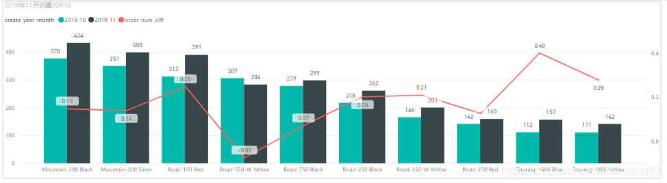
2019年11月TOP10销量品牌情况
-
根据图可以看出:
- (1)Mountain-200 Black 品牌2019年11月销量最多,为434台;
- (2)2019年11月销量TOP10的品牌中仅Road-550-W Yellow 销量环比为负数,其余均为正增长;
- (3)2019年11月销量TOP10的品牌中Touring-1000 Blue 、Touring-1000 Yellow和Road-150 Red 三个品牌增速较高,在25%以上
-
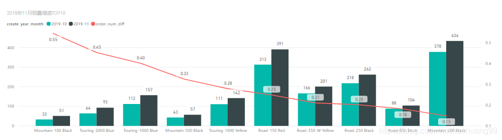
2019年11月TOP10销量环比品牌情况
-
根据图可以看出:
- (1)Mountain-100 Black品牌2019年11月环比最高,为55%;
- (2)2019年11月销量环比TOP10的品牌中最低为Mountain-200 Black,环比为15%;
- (3)2019年11月TOP10销量和TOP10增速中,有Touring-1000 Blue、Touring-1000 Yellow、Road-150 Red、Road-350-W Yellow和Road-250 Black同时占有一席之地
四、总结
- 本项目数据量在10万+条,通过python、mysql与PoweBI的联动使用,熟练操作;
- 本次分析由浅入深,从多个角度出发对数据进行剖析,较好的利用数据资料;
- 目前只进行初级的数据分析和可视化展示,后续需要搭建PowerBI看板和自动化更新展示界面,对数据分析的学习还有待深入


 501
501


 被折叠的 条评论
为什么被折叠?
被折叠的 条评论
为什么被折叠?
 到【灌水乐园】发言


