Little's Law: Latency & Throughput-CSDN博客

I’ve been doing a lot of analysis of latency and throughput recently as a part of benchmarking work on databases. I thought I’d share some insights on how the two are related. For an overview of what these terms mean, check out Aater’s post describing the differences between them here.

In this post we’ll talk about how they each relate to one another.

The basic relationship between latency and throughput within a stable system—one that is not ramping up and down—is defined by a simple equation called Little’s Law:

occupancy = latency x throughput

Latency in this equation means the unloaded latency of the system, plus the queuing time that Aater wrote about in the post referenced above. Occupancy is the number of requestors in the system.

The Water Pipe Revisited

To understand the latency/throughput relationship, let’s go back to Aater’s example of the water pipe.

Occupancy is the amount of water in the pipe through which we are measuring latency and throughput. The throughput is the rate at which water leaves the pipe, and the latency is the time it takes to get water from one end of the pipe to the other.

If we cut the pipe in two, we halve the latency, but throughput remains constant. That’s because by halving the water pipe we’ve also halved the total amount of water in the pipe. On the other hand, if we add another pipe, the latency is unaffected and the throughput is doubled because the amount of water in the system has doubled. Increasing the water pressure also changes the system. If we double the speed at which the water travels we halve the latency, double the throughput, and the occupancy remains constant.

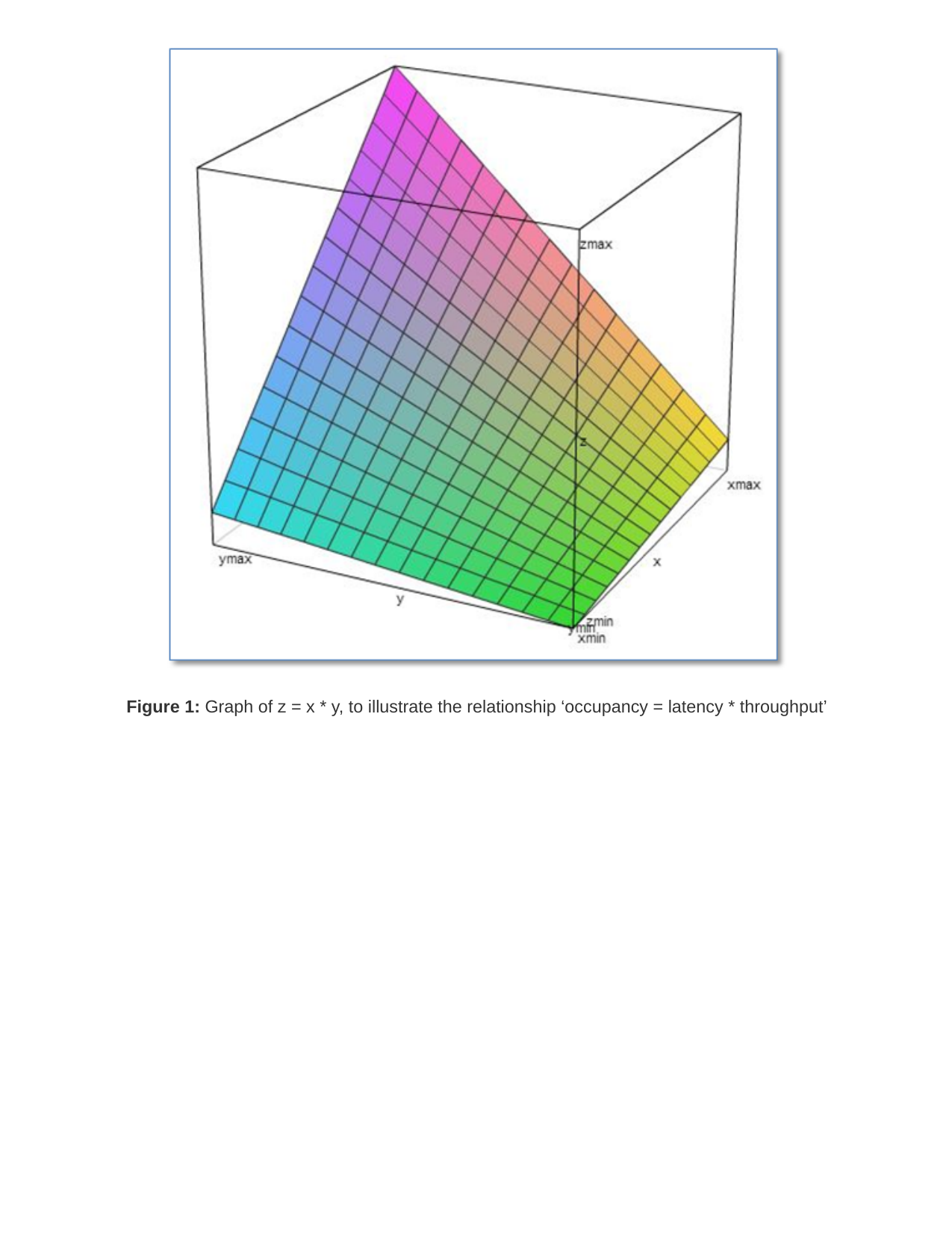
The following figures give a graphical view of the equation.

Figure 1: Graph of z = x * y, to illustrate the relationship ‘occupancy = latency * throughput’

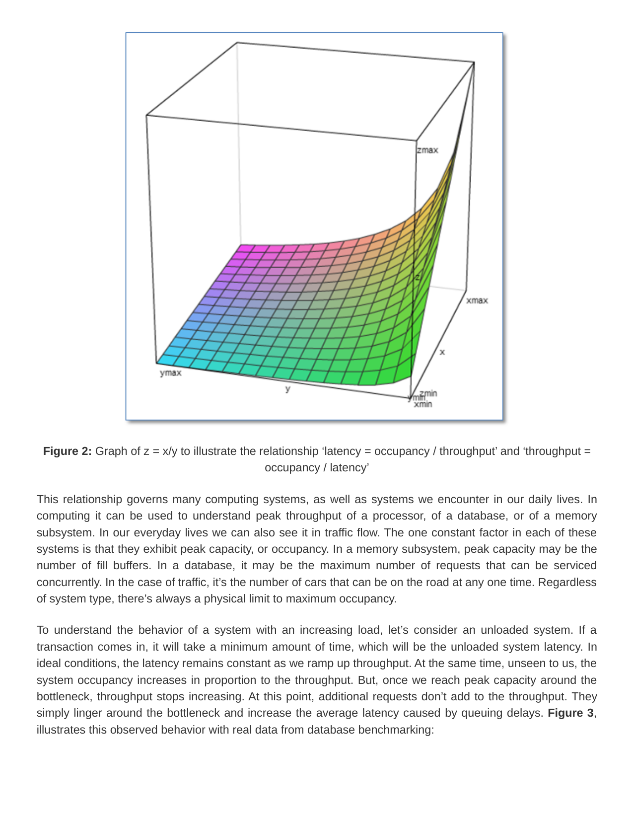
Figure 2: Graph of z = x/y to illustrate the relationship ‘latency = occupancy / throughput’ and ‘throughput = occupancy / latency’

This relationship governs many computing systems, as well as systems we encounter in our daily lives. In computing it can be used to understand peak throughput of a processor, of a database, or of a memory subsystem. In our everyday lives we can also see it in traffic flow. The one constant factor in each of these systems is that they exhibit peak capacity, or occupancy. In a memory subsystem, peak capacity may be the number of fill buffers. In a database, it may be the maximum number of requests that can be serviced concurrently. In the case of traffic, it’s the number of cars that can be on the road at any one time. Regardless of system type, there’s always a physical limit to maximum occupancy.

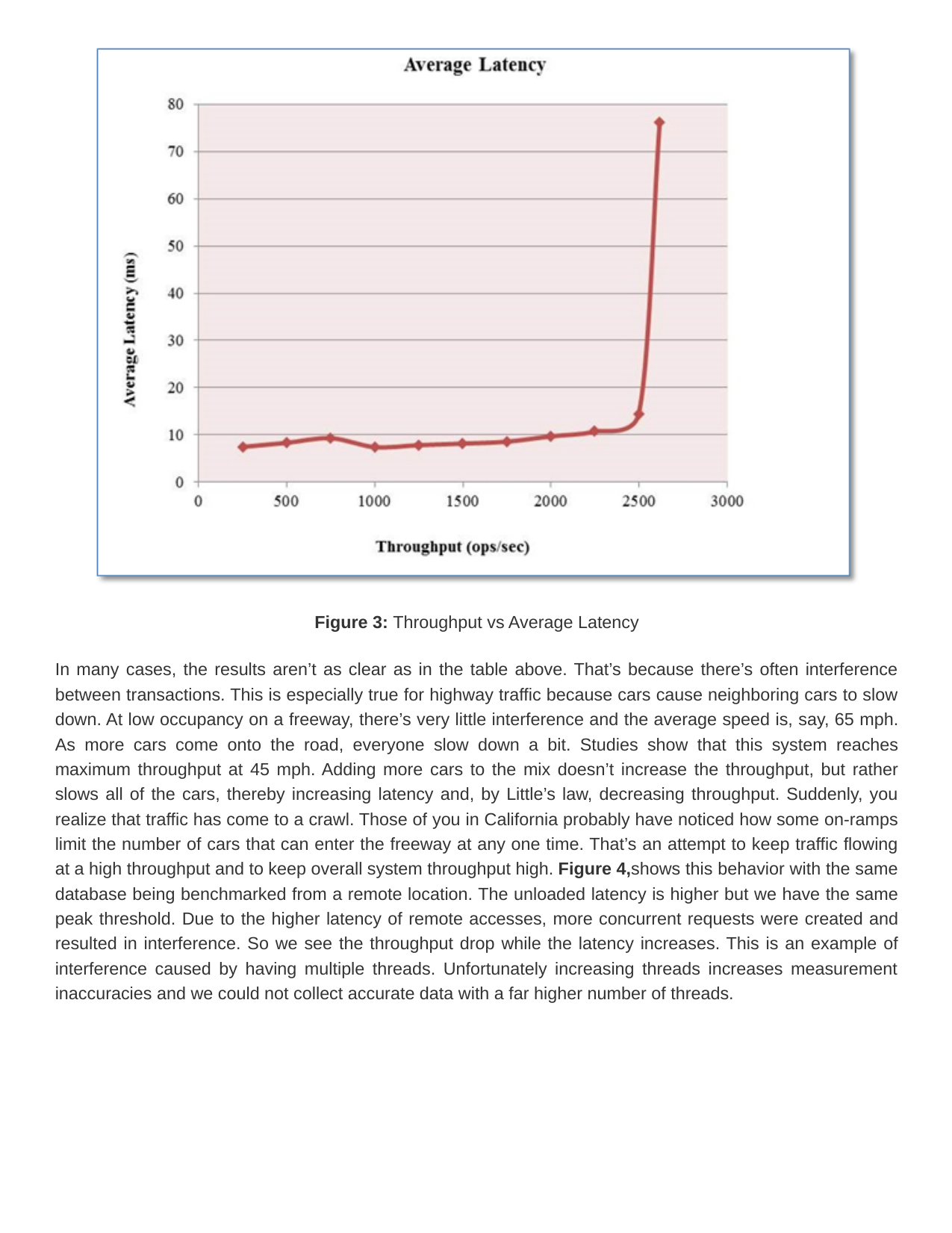
To understand the behavior of a system with an increasing load, let’s consider an unloaded system. If a transaction comes in, it will take a minimum amount of time, which will be the unloaded system latency. In ideal conditions, the latency remains constant as we ramp up throughput. At the same time, unseen to us, the system occupancy increases in proportion to the throughput. But, once we reach peak capacity around the bottleneck, throughput stops increasing. At this point, additional requests don’t add to the throughput. They simply linger around the bottleneck and increase the average latency caused by queuing delays. Figure 3, illustrates this observed behavior with real data from database benchmarking:

Figure 3: Throughput vs Average Latency

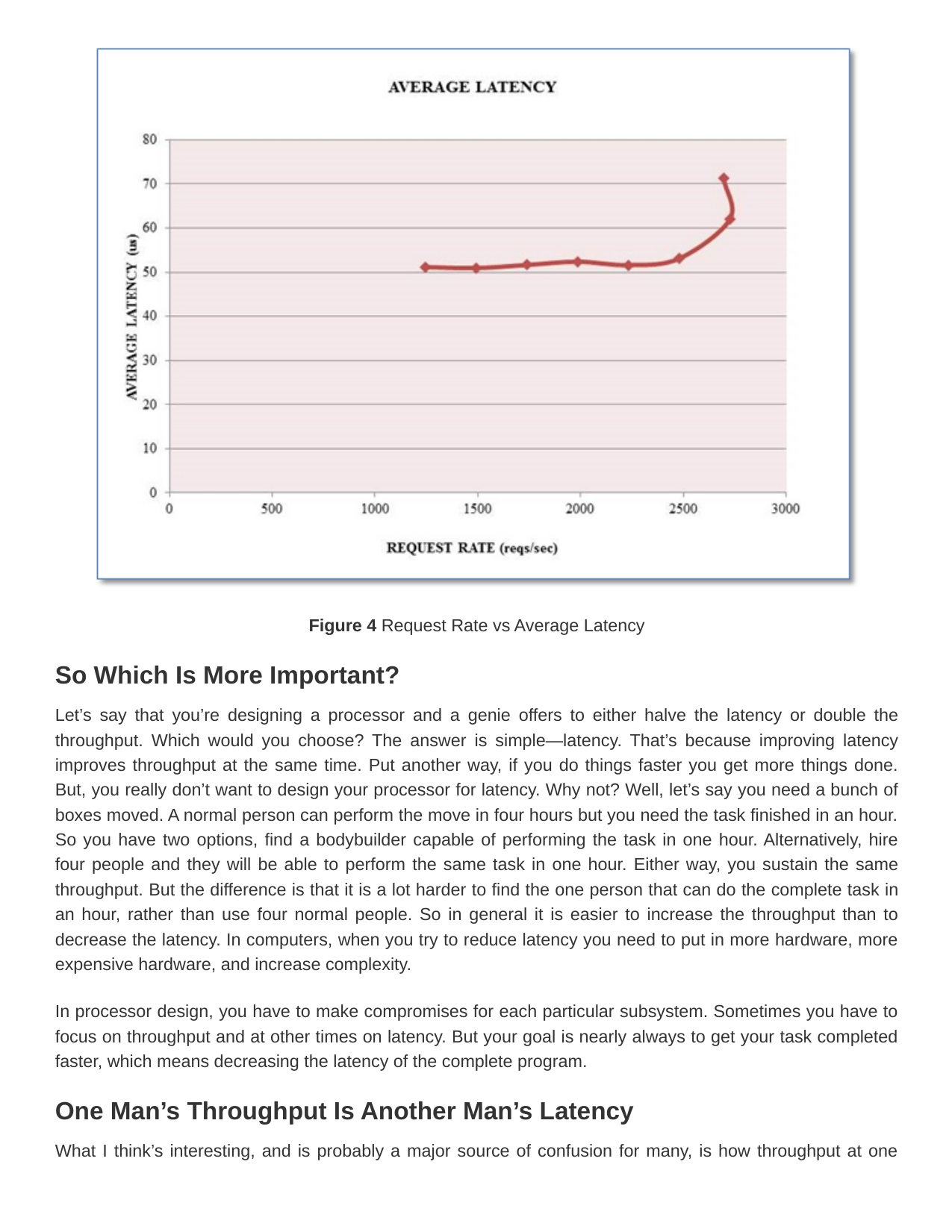
In many cases, the results aren’t as clear as in the table above. That’s because there’s often interference between transactions. This is especially true for highway traffic because cars cause neighboring cars to slow down. At low occupancy on a freeway, there’s very little interference and the average speed is, say, 65 mph. As more cars come onto the road, everyone slow down a bit. Studies show that this system reaches maximum throughput at 45 mph. Adding more cars to the mix doesn’t increase the throughput, but rather slows all of the cars, thereby increasing latency and, by Little’s law, decreasing throughput. Suddenly, you realize that traffic has come to a crawl. Those of you in California probably have noticed how some on-ramps limit the number of cars that can enter the freeway at any one time. That’s an attempt to keep traffic flowing at a high throughput and to keep overall system throughput high. Figure 4, shows this behavior with the same database being benchmarked from a remote location. The unloaded latency is higher but we have the same peak threshold. Due to the higher latency of remote accesses, more concurrent requests were created and resulted in interference. So we see the throughput drop while the latency increases. This is an example of interference caused by having multiple threads. Unfortunately increasing threads increases measurement inaccuracies and we could not collect accurate data with a far higher number of threads.

Figure 4 Request Rate vs Average Latency

So Which Is More Important?

Let’s say that you’re designing a processor and a genie offers to either halve the latency or double the throughput. Which would you choose? The answer is simple—latency. That’s because improving latency improves throughput at the same time. Put another way, if you do things faster you get more things done. But, you really don’t want to design your processor for latency. Why not? Well, let’s say you need a bunch of boxes moved. A normal person can perform the move in four hours but you need the task finished in an hour. So you have two options, find a bodybuilder capable of performing the task in one hour. Alternatively, hire four people and they will be able to perform the same task in one hour. Either way, you sustain the same throughput. But the difference is that it is a lot harder to find the one person that can do the complete task in an hour, rather than use four normal people. So in general it is easier to increase the throughput than to decrease the latency. In computers, when you try to reduce latency you need to put in more hardware, more expensive hardware, and increase complexity.

In processor design, you have to make compromises for each particular subsystem. Sometimes you have to focus on throughput and at other times on latency. But your goal is nearly always to get your task completed faster, which means decreasing the latency of the complete program.

One Man’s Throughput Is Another Man’s Latency

What I think’s interesting, and is probably a major source of confusion for many, is how throughput at one level determines latency at the next higher level. The simplest example of this is an instruction. We can design a processor that wastes no time in latching the results and that executes an instruction in one long cycle. But we don’t because we can get much higher throughput by pipelining the instructions, while causing only a nominal increase in latency due to the additional time taken to latch the results. So, by increasing single-instruction latency we decrease the latency of processing a complete stream of instructions.

A 1-cycle processor versus a pipelined processor is an extreme case, but it represents a real-life compromise. For multiple parallel data streams, you can ignore CPUs that are designed for reducing latency on a single data stream. Instead, you can use a GPU that executes a single data stream at a significantly slower speed, but processes multiple streams in parallel in order to complete the task at a faster overall speed.

Yet, there are higher levels still. If you don’t need to run your operation on a single system, you can use clusters of multiple systems. When using parallelism to increase throughput, you have to ask yourself the same question that you ask when looking at any parallelism problem: What are the data dependencies and how much data will need to be shared?

The relationship between latency and throughput across different levels can be confusing. It’s a reminder that we need to look at each system as a whole. Any system we see in real life will include many subsystems, and there will be complex dependencies between them. Each subsystem will bind to the rest of the system, either by throughput or by latency. When designing a system, it’s important to consider these interactions and then to create a system that won’t bottleneck the larger system. These same rules apply to everything, including supply chains, CPU performance, databases and highway traffic. So, when asking yourself which is fastest, first ask what fast means for you in terms of latency and throughput, and how your system meets these goals.