


day 3
文章目录
3.1梯度下降法求最小值公式推导、代码及动画展示
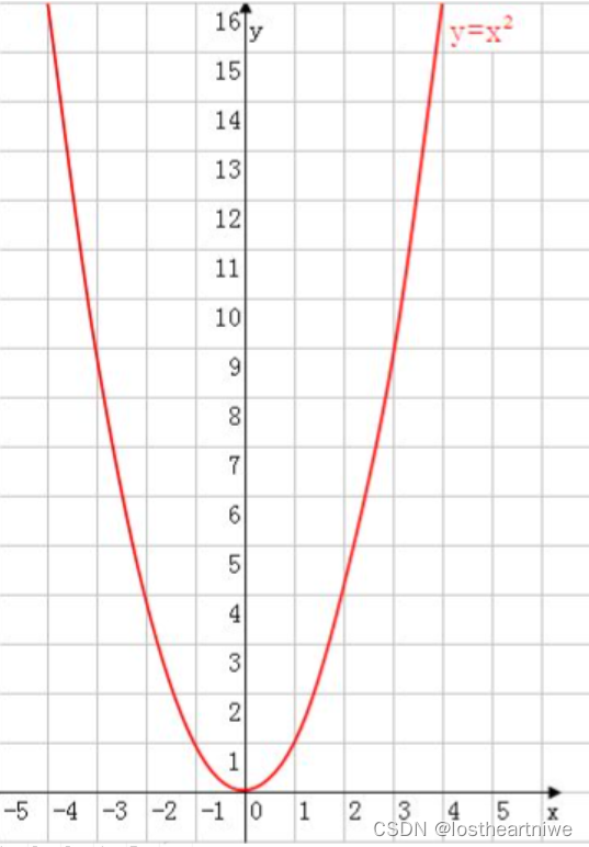
y=x^2求最小值
梯度下降法求值
代码部分:
import numpy as np


# 定义函数 y = x^2
def f(x):
    return x ** 2


# 定义梯度函数 df/dx = 2x
def df(x):
    return 2 * x


# 初始化参数
x = 5.0  # 初始点,可以选择其他值
learning_rate = 0.1  # 学习率,控制每次更新的步长
epsilon = 1e-7  # 收敛阈值,当梯度小于这个值时停止迭代
max_iterations = 1000  # 最大迭代次数

# 梯度下降过程
for i in range(max_iterations):
    grad = df(x)  # 计算当前点的梯度
    if abs(grad) < epsilon:  # 如果梯度小于阈值,则停止迭代
        break
    x -= learning_rate * grad  # 更新 x 的值
    print(f"Iteration {i + 1}: x = {x}, y = {f(x)}")

print(f"Found minimum at x = {x}, y = {f(x)}")
运行结果:
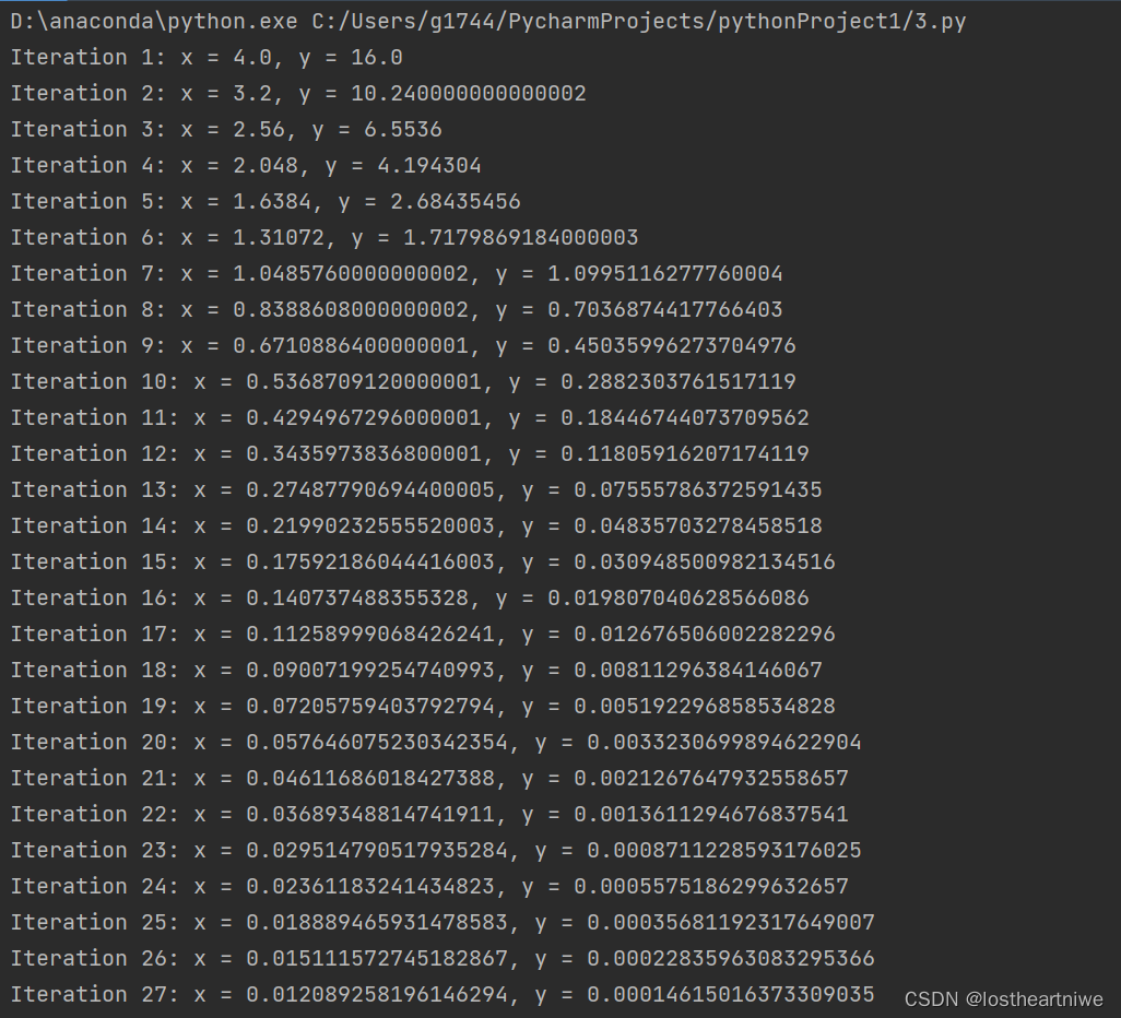
我只截了一部分运行结果
运行原理:
首先,要明确一点,梯度下降法通常用于求解函数的极值,特别是当函数没有显式解或者求解过程非常复杂时。对于函数y = x^2,其最小值是非常直观的,即当x = 0时,y取得最小值0。
但为了满足需求,仍然可以使用梯度下降法来求解这个函数的最小值。梯度下降法的核心思想是通过迭代的方式,沿着函数梯度的反方向更新参数,从而逐渐逼近函数的最小值。
对于函数y = x^2,其梯度(即导数)为*{dy}/{dx} = 2x。*在梯度下降法中,我们选择一个初始点x_0,然后按照以下公式进行迭代:
x_{n+1} = x_n - a *{dy}/{dx}
其中,a是学习率,它决定了每次迭代的步长。如果a太大,可能会导致迭代过程不稳定;如果a太小,则可能导致迭代速度过慢。
3.2梯度下降法求线性回归公式、代码及动画
代码:
import numpy as np
import matplotlib

matplotlib.use('TkAgg')  # 或者使用其他交互式后端,如 'Qt5Agg'
import matplotlib.pyplot as plt

plt.rcParams['font.sans-serif'] = ['SimHei']  # 使用黑体
plt.rcParams['axes.unicode_minus'] = False  # 正确显示负号

# 数据
x = np.array([0.18, 0.1, 0.16, 0.08, 0.09, 0.11, 0.12, 0.17, 0.15, 0.14, 0.13])
y = np.array([0.18, 0.1, 0.16, 0.08, 0.09, 0.11, 0.12, 0.17, 0.15, 0.14, 0.13])

# 初始化参数
lr = 2.5  # 学习率
w = 10
epochs = 50  # 修改拼写错误

# 初始化列表来保存每次迭代的梯度、权重和损失
gradients = []
weights = [w]
losses = []

# 初始化图形和子图
plt.figure(figsize=(12, 9))

# 初始化子图
gradient_plot = plt.subplot(3, 1, 1)
weight_plot = plt.subplot(3, 1, 2)
loss_plot = plt.subplot(3, 1, 3)

# 梯度下降算法
for i in range(epochs):
    ya = w * x
    loss = 1 / 2.0 * np.sum((ya - y) ** 2)
    w_gar = np.mean((ya - y) * x)
    w = w - lr * w_gar

    # 保存梯度、权重和损失
    gradients.append(w_gar)
    weights.append(w)
    losses.append(loss)

    # 更新图形数据
    gradient_plot.clear()
    gradient_plot.plot(gradients)
    weight_plot.clear()
    weight_plot.plot(weights)
    loss_plot.clear()
    loss_plot.plot(losses)

    # 设置子图的标题和标签
    gradient_plot.set_title('梯度随时间的变化')
    gradient_plot.set_xlabel('迭代次数')
    gradient_plot.set_ylabel('梯度')
    weight_plot.set_title('权重随时间的变化')
    weight_plot.set_xlabel('迭代次数')
    weight_plot.set_ylabel('权重')
    loss_plot.set_title('损失随时间的变化')
    loss_plot.set_xlabel('迭代次数')
    loss_plot.set_ylabel('损失')

    # 绘制网格
    gradient_plot.grid(True)
    weight_plot.grid(True)
    loss_plot.grid(True)

    # 绘制当前迭代的信息
    plt.draw()
    plt.pause(0.5)  # 暂停一段时间以便可以看到图形更新
# 调整子图参数
plt.subplots_adjust(hspace=0.8, wspace=0.7)
# 显示图形(在循环结束后)
plt.tight_layout()
plt.ioff()  # 关闭交互模式,以避免图形在关闭时卡住
plt.show()
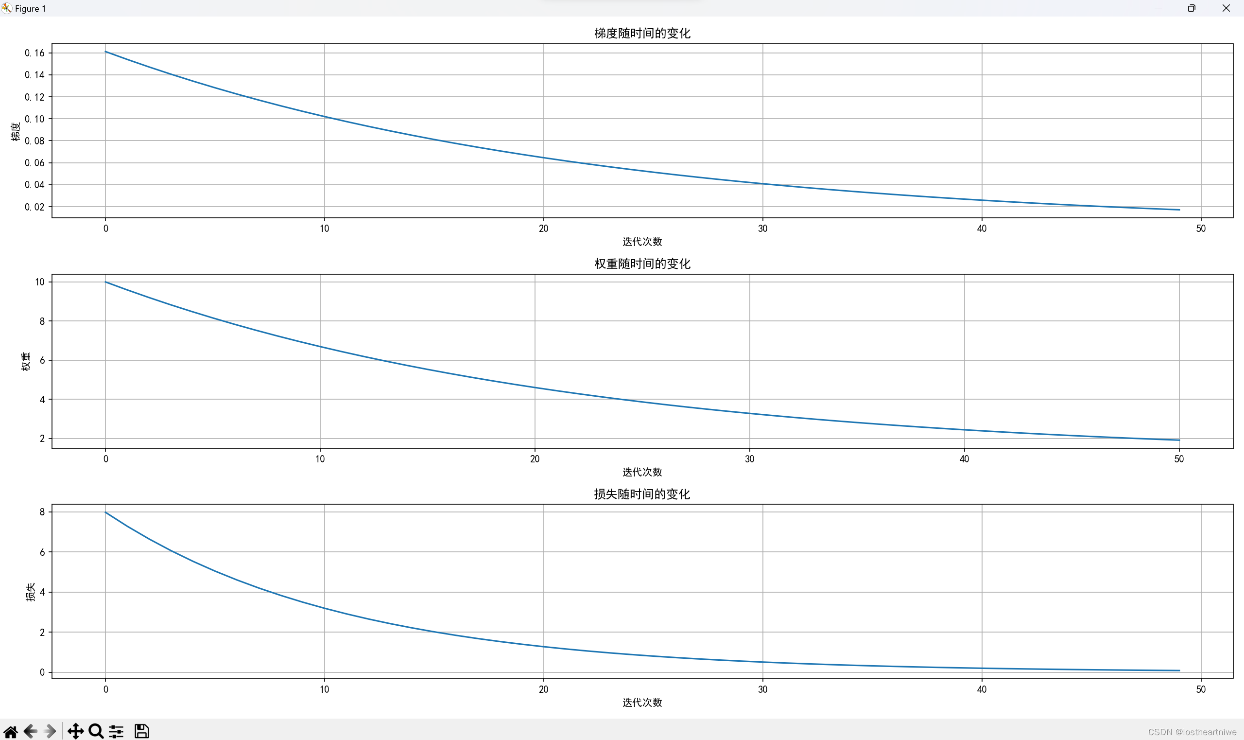
运行结果:
3.3利用pytorch(一)顺序结构实现梯度下降拟合线性回归
代码:
import matplotlib
matplotlib.use('TkAgg') # 或者 'Qt5Agg', 'WXAgg' 等,取决于你的系统
import matplotlib.pyplot as plt
import torch
####################顺序结构实现梯度下降拟合线性回归######################
x_data = torch.tensor([[0.18], [0.1], [0.16], [0.08], [0.09], [0.11], [0.12], [0.17], [0.15], [0.14]])
y_data = torch.tensor([[0.18], [0.1], [0.16], [0.08], [0.09], [0.11], [0.12], [0.17], [0.15], [0.14]])
# 2 定义参数
w = torch.tensor([[10]], requires_grad=True, dtype=torch.float32) # 定义权重参数
b = torch.tensor([0], requires_grad=True, dtype=torch.float32)
learning_rate = 0.5 # 定义学习率
epoch = 5000
# 3 通过循环迭代逼近w与b的值,也就是更新w,b参数,倒数是通过反向传播求导得到
for i in range(epoch):
y_predict = torch.matmul(x_data, w)+b # 模型 正向传播
loss = (y_data - y_predict).pow(2).mean() # 计算 均方差 loss函数
if w.grad is not None:
w.grad.data.zero_() # 对参数w与b的gard进行归零,然后在反向传播
if b.grad is not None:
b.grad.data.zero_()
loss.backward() # 模型反向传播 得到w,b的倒数(梯度)
w.data = w.data - learning_rate * w.grad # 更新模型中的权重参数
b.data = b.data - learning_rate * b.grad
print("w ,b ,loss", w.item(), b.item(), loss.item(), i)
print("最终的: w,b ,loss", w.item(), b.item(), loss.item(), i)
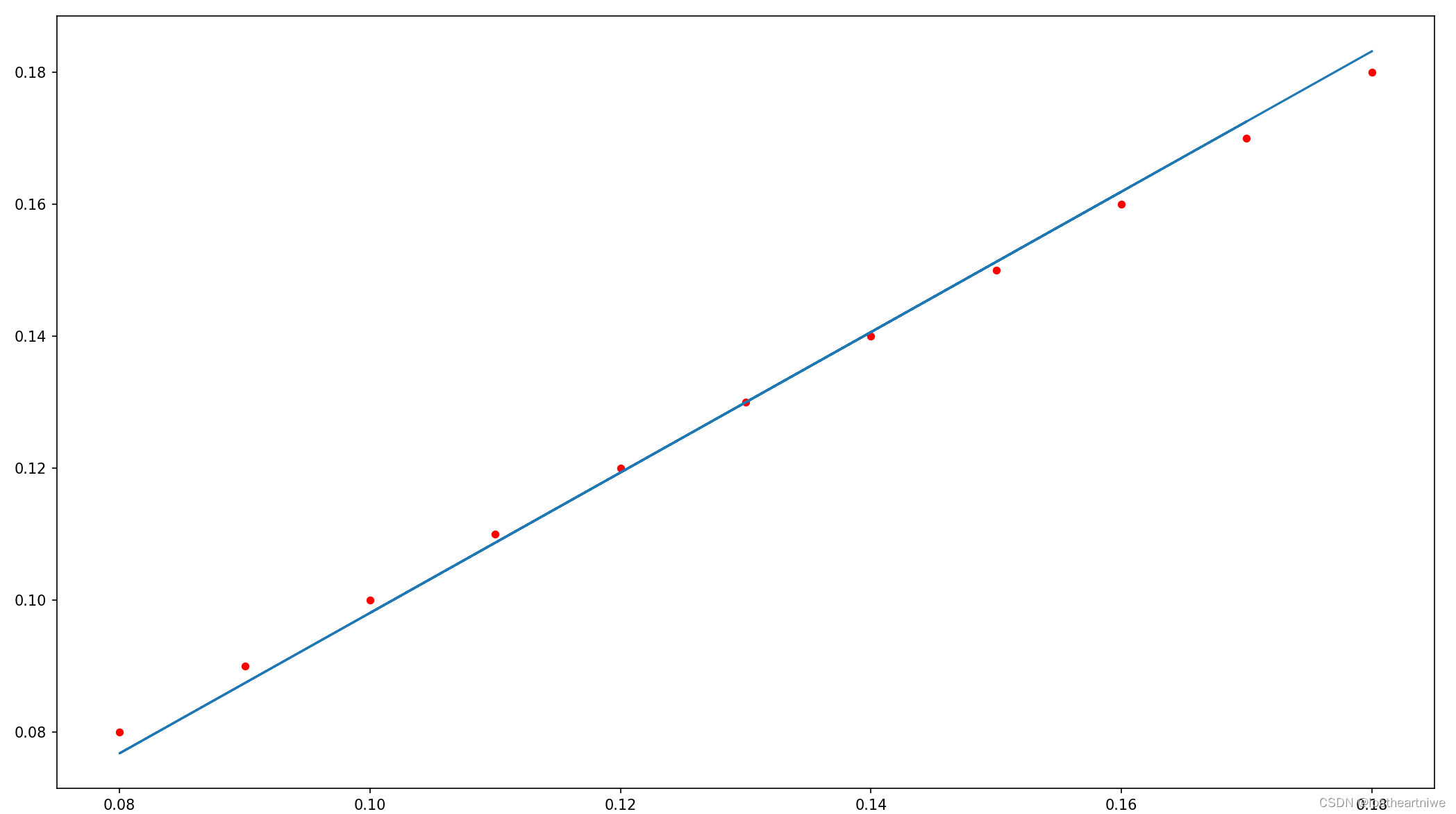
# 可视化 真实数据用红点-scatter(),预测数据用直线蓝色-polt()
plt.figure()
plt.scatter(x_data, y_data, 20, 'r')
y_predict = torch.matmul(x_data, w) + b
plt.plot(x_data, y_predict.detach().numpy())
plt.show()
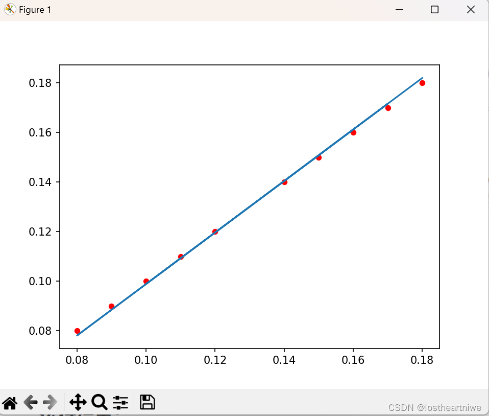
运行结果:
3.4利用pytorch(二)封装类实现梯度下降拟合线性回归
代码部分:
import matplotlib
matplotlib.use('TkAgg') # 或者 'Qt5Agg', 'WXAgg' 等,取决于你的系统
import torch
import matplotlib.pyplot as plt
################# 第2种方法 利用pytorch封装类实现梯度下降拟合线性回归 #########
class LModel:
# 构造函数初始化
def __init__(self, learning_rate):
self.w = torch.tensor([[10]], requires_grad=True, dtype=torch.float32) # 定义权重参数
self.b = torch.tensor([0], requires_grad=True, dtype=torch.float32)
self.learning_rate = learning_rate
self.loss = None
# 前馈函数forward,对父类函数中的overwrite
def forward(self, x, y):
# 调用linear中的call(),以利用父类forward()计算wx+b
y_pred = torch.matmul(x, self.w) + self.b
self.loss = (y - y_pred).pow(2).mean()
return y_pred
def backward(self):
if self.w.grad is not None:
self.w.grad.data.zero_()
if self.b.grad is not None:
self.b.grad.data.zero_()
self.loss.backward()
self.w.data = self.w.data - self.learning_rate * self.w.grad # 更新模型中的权重参数
self.b.data = self.b.data - self.learning_rate * self.b.grad
print("最终的:w ,b ,loss", self.w.item(), self.b.item(), self.loss.item())
x_data = torch.tensor([[0.18], [0.1], [0.16], [0.08], [0.09], [0.11], [0.12], [0.17], [0.15], [0.14], [0.13]])
y_data = torch.tensor([[0.18], [0.1], [0.16], [0.08], [0.09], [0.11], [0.12], [0.17], [0.15], [0.14], [0.13]])
epoch = 5000
model = LModel(learning_rate=0.5)
for i in range(epoch):
model.forward(x_data, y_data)
model.backward()
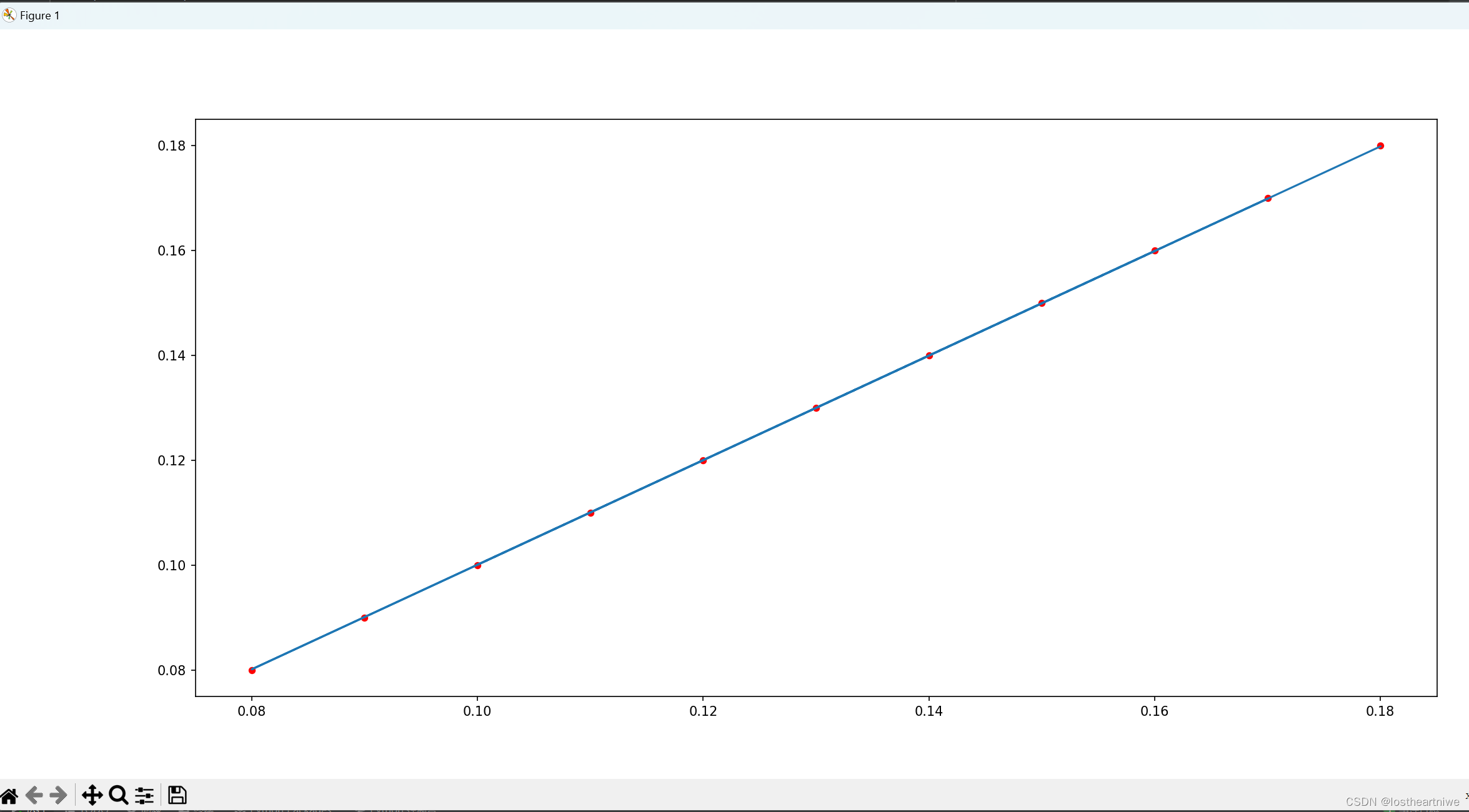
# 可视化 真实数据用点红色-scatter(),预测数据用直线蓝色-plot()
plt.figure(figsize=(20, 8))
plt.scatter(x_data, y_data, 20, 'r')
y_predict = model.forward(x_data, y_data)
plt.plot(x_data, y_predict.detach().numpy())
plt.show()
运行结果:
3.5利用pytorch(三)继承类实现梯度下降拟合线性回归
代码部分:
import torch
import matplotlib

matplotlib.use('TkAgg')  # 或者 'Qt5Agg', 'WXAgg' 等,取决于你的系统
import matplotlib.pyplot as plt

############# 第3种方法 利用pytorch继承类实现梯度下降拟合线性回归#######################

# 固定继承于Module
class LinearModel(torch.nn.Module):
    # 构造函数初始化
    def __init__(self):
        # 调用父类的init
        super(LinearModel, self).__init__()
        # y = weight(w) * x + bias(b)
        # torch.nn.Linear(in_features, out_features, bias=True)
        self.linear = torch.nn.Linear(1, 1)

    # 前馈函数forward,对父类函数中的overwrite
    def forward(self, x):
        # 调用linear中的call(),以利用父类forward()计算wx+b
        y_pred = self.linear(x)
        return y_pred
    # 反馈函数backward由module自动根据计算图生成

# 定义数据集
x_data = torch.Tensor([[0.18], [0.1], [0.16], [0.08], [0.09], [0.11], [0.12], [0.17], [0.15], [0.14], [0.13]])
y_data = torch.Tensor([[0.18], [0.1], [0.16], [0.08], [0.09], [0.11], [0.12], [0.17], [0.15], [0.14], [0.13]])

# 定义模型
model = LinearModel()

# 构造 均方差 损失函数
#criterion = torch.nn.MSELoss(size_average=False)
criterion = torch.nn.MSELoss(reduction='sum')
# 使用梯度下降法进行优化
optimizer = torch.optim.SGD(model.parameters(), lr=0.05)

for epoch in range(5000):
    y_pred = model(x_data)            # 前向传播计算y_pred
    loss = criterion(y_pred, y_data)  # 前馈计算损失loss
    optimizer.zero_grad()             # 梯度清零
    loss.backward()                   # 梯度反向传播,计算图清除
    optimizer.step()                  # 根据传播的梯度以及学习率更新参数
    print(loss)
    # 根据传播的梯度以及学习率更新参数
# 输出模型权重值
print('w = ', model.linear.weight.item())
print('b = ', model.linear.bias.item())

# 预测值
x_test = torch.Tensor([[4.0]])
y_test = model(x_test)
print('y_pred = ', y_test.data)

# 可视化 真实数据用点红色-scatter(),预测数据用直线蓝色-plot()
plt.figure(figsize=(20, 8))
plt.scatter(x_data, y_data, 20, 'r')
y_predict = model(y_data)
plt.plot(x_data, y_predict.detach().numpy())
plt.show()
报错部分:
在运行过程中,虽然能够运行出来,运行没有任何问题,但还是会报错,报错原因是
UserWarning: size_average and reduce args will be deprecated, please use reduction='sum' instead.
  warnings.warn(warning.format(ret))
修改过后源代码改为现在代码
criterion = torch.nn.MSELoss(size_average=False)
改为
criterion = torch.nn.MSELoss(reduction='sum')
原因:
在 PyTorch 的神经网络模块(
torch.nn)中,size_average和reduce这两个参数将会在将来的版本中不再被使用,并建议你使用新的参数reduction来代替它们。reduction参数可以接受'sum'或'mean'作为值,分别对应求和和求平均值。
运行结果:


 5万+
5万+


 被折叠的 条评论
为什么被折叠?
被折叠的 条评论
为什么被折叠?
 到【灌水乐园】发言


