机器学习sklearn19.0——集成学习——boosting与梯度提升算法（GBDT）、Adaboost算法

一、boosting算法原理

二、梯度提升算法

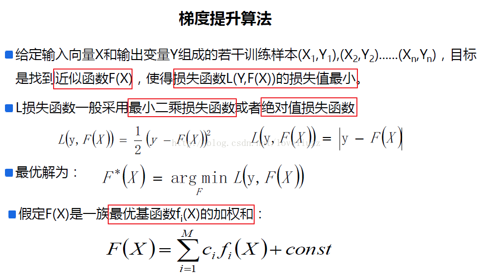
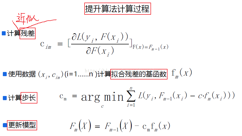
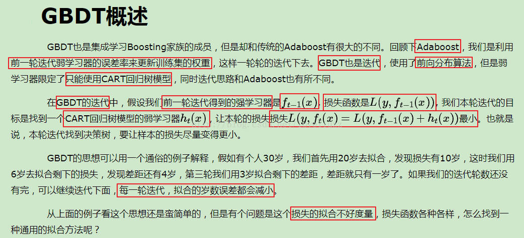
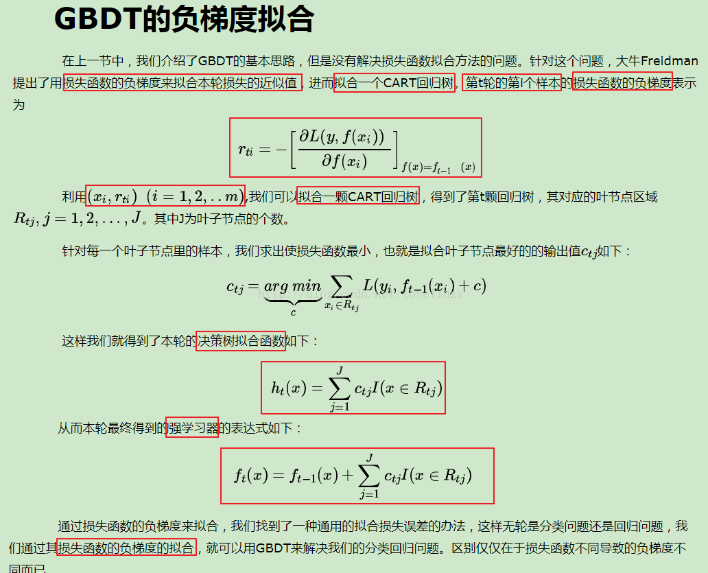
关于提升梯度算法的详细介绍，参照博客：http://www.cnblogs.com/pinard/p/6140514.html

对该算法的sklearn的类库介绍和调参，参照网址：http://www.cnblogs.com/pinard/p/6143927.html

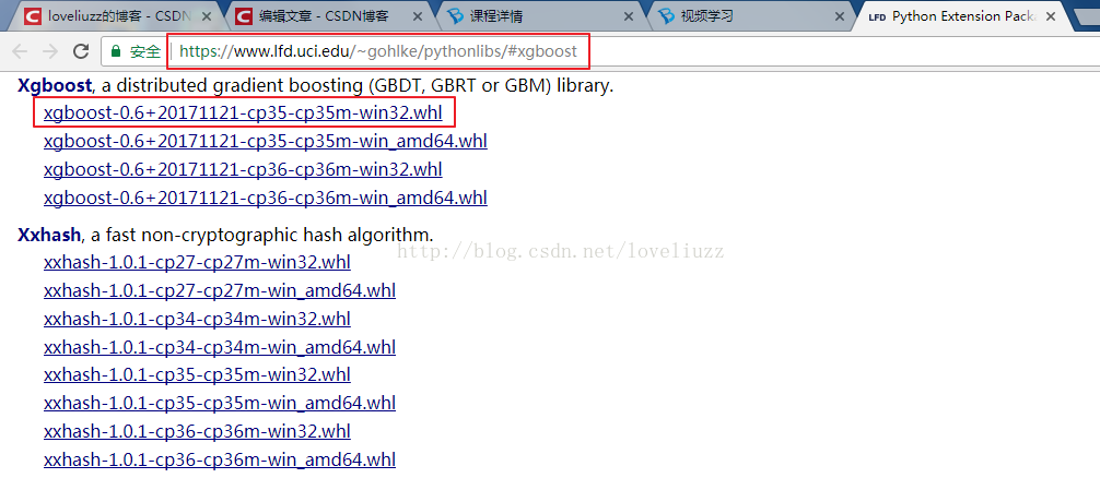
xgboost安装

（1）在网址    https://www.lfd.uci.edu/~gohlke/pythonlibs/#xgboost   中下载相应的版本

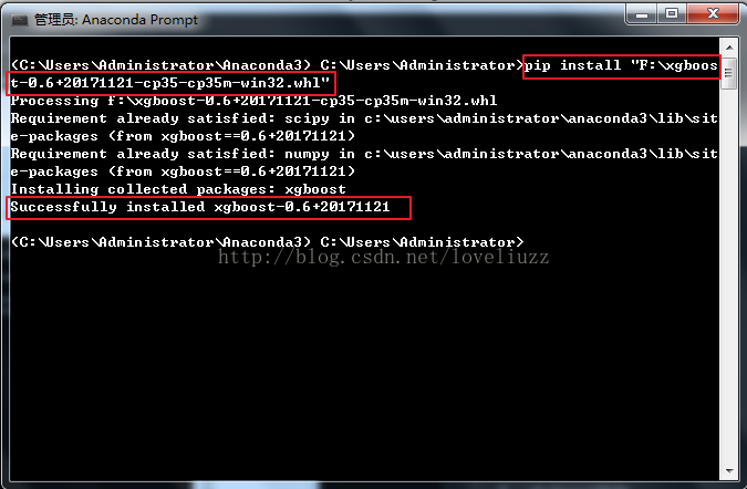
（2）在anaconda prompt中安装

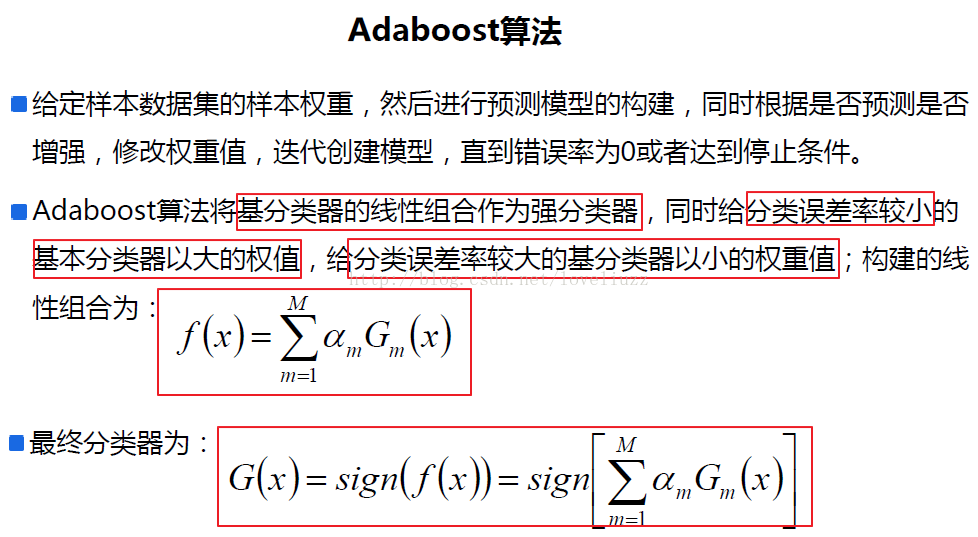
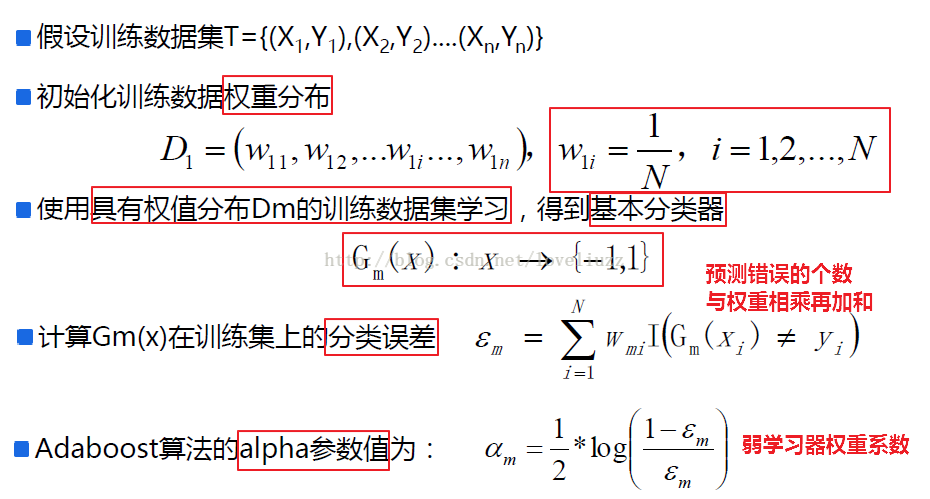
三、adaboost算法

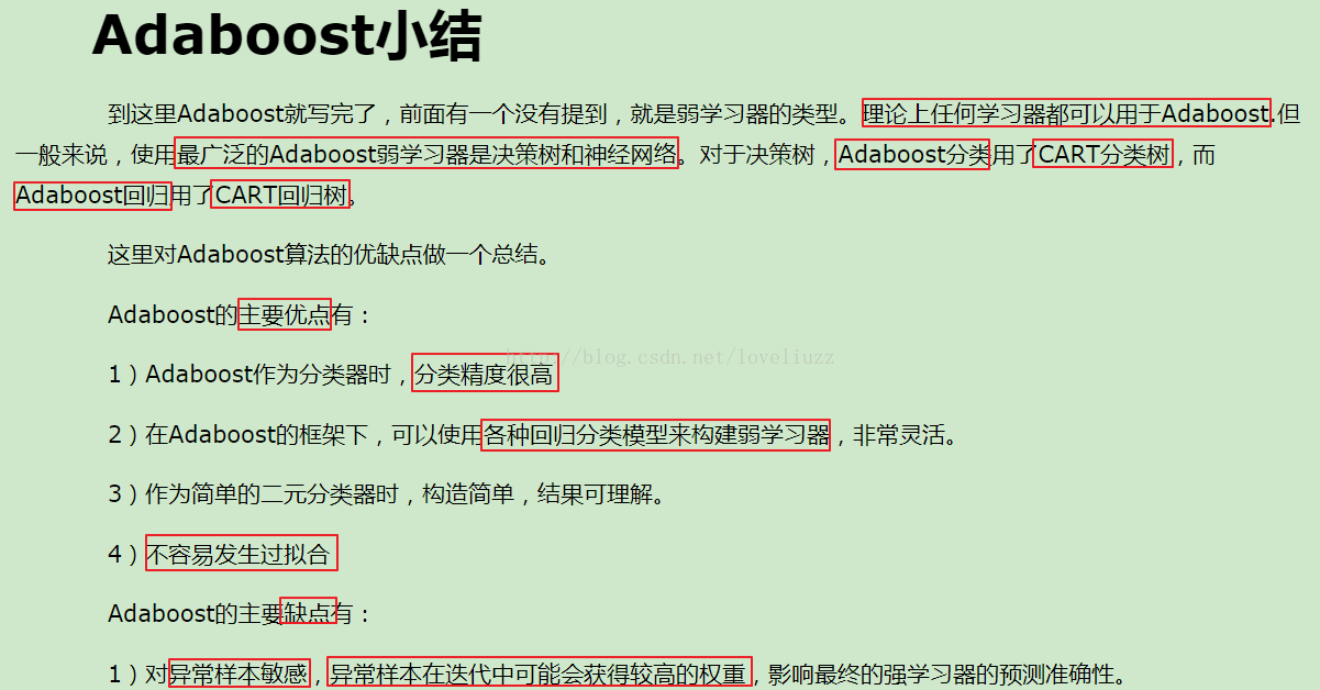
注：adaboost算法详细介绍参照博客地址：http://www.cnblogs.com/pinard/p/6133937.html

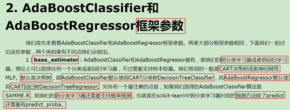
四、adaboost算法类库介绍

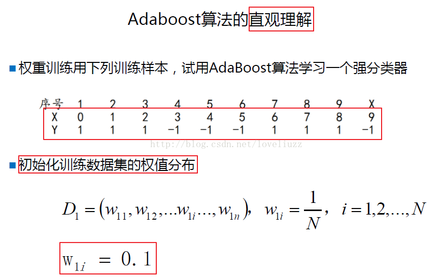
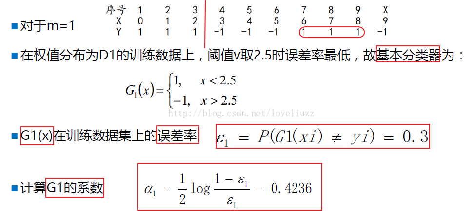
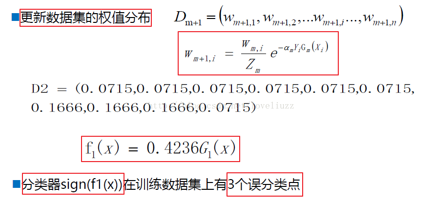
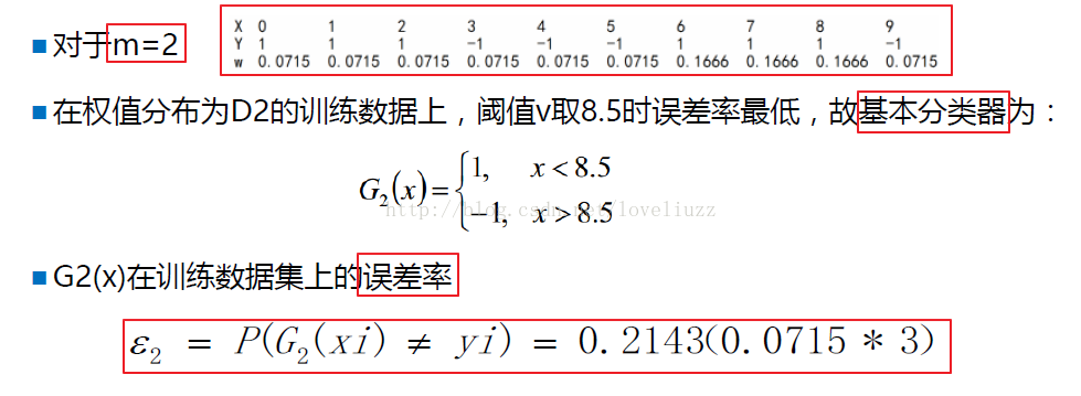
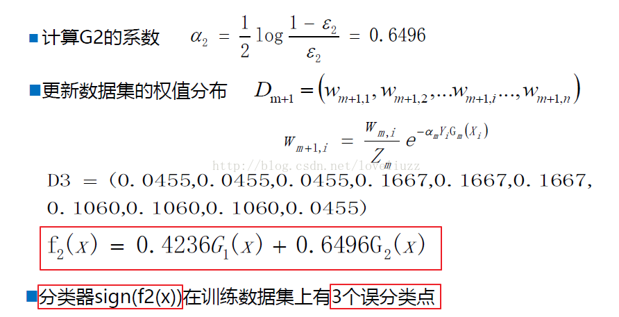
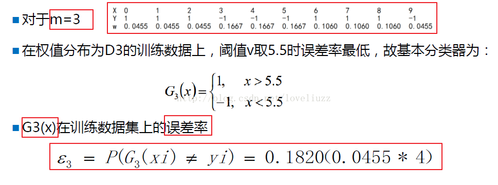
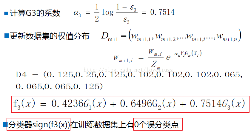
五、adaboost算法示例举例

（1）知识点介绍

（2）示例代码

#!/usr/bin/env python
# -*- coding:utf-8 -*-
# Author:ZhengzhengLiu

#Adaboost算法

from sklearn.ensemble import AdaBoostClassifier
from sklearn.tree import DecisionTreeClassifier
from sklearn.datasets import make_gaussian_quantiles
import numpy as np
import matplotlib as mpl
import matplotlib.pyplot as plt

#解决中文显示问题
mpl.rcParams['font.sans-serif']=[u'simHei']
mpl.rcParams['axes.unicode_minus']=False

#创建数据
#生成2维正态分布，生成的数据按分位数分为两类，200个样本,2个样本特征，协方差系数为2
X1,y1 = make_gaussian_quantiles(cov=2,n_samples=200,n_features=2,
                                n_classes=2,random_state=1) #创建符合高斯分布的数据集
X2,y2 = make_gaussian_quantiles(mean=(3,3),cov=1.5,n_samples=300,n_features=2,
                                n_classes=2,random_state=1)
#将两组数据合成一组数据
X = np.concatenate((X1,X2))
y = np.concatenate((y1,-y2+1))

#构建adaboost模型
bdt = AdaBoostClassifier(DecisionTreeClassifier(max_depth=1),
                         algorithm="SAMME.R",n_estimators=200)

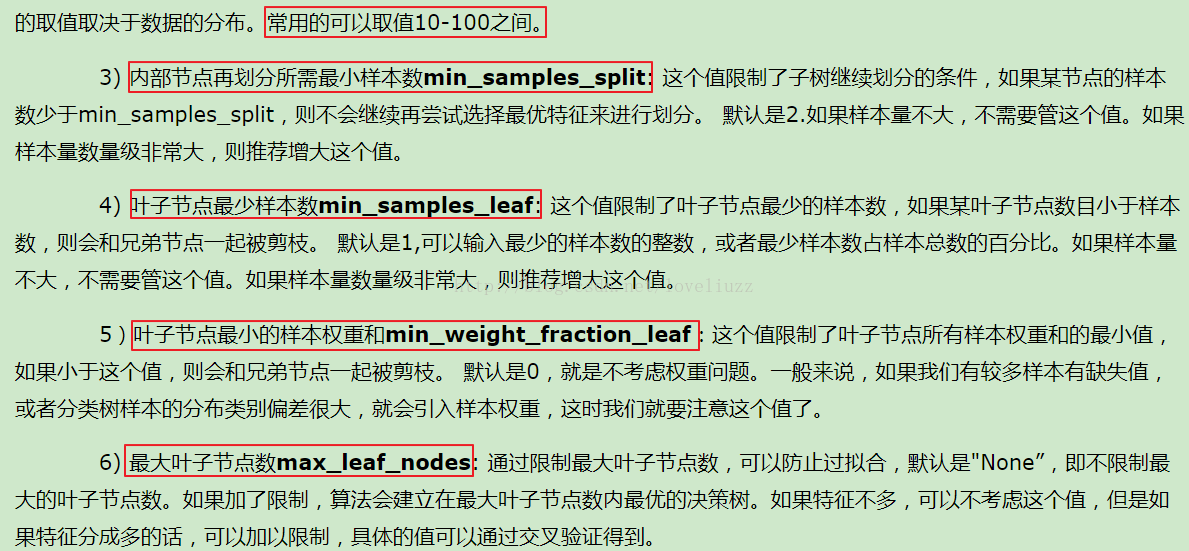
#数据量大时，可以增加内部分类器的max_depth(树深)，也可不限制树深，树深的范围为：10-100
#数据量小时，一般可以设置树深较小或者n_estimators较小
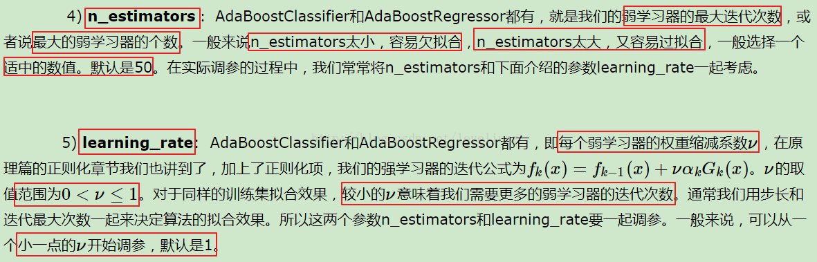
#n_estimators:迭代次数或最大弱分类器数
#base_estimator:DecisionTreeClassifier，选择弱分类器，默认为CART树
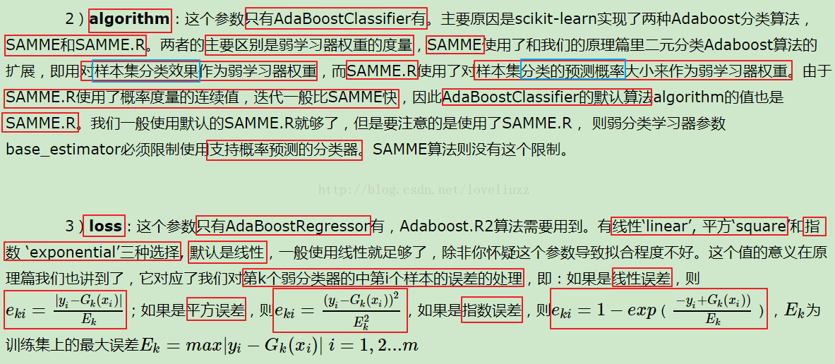
#algorithm：SAMME和SAMME.R，运算规则，后者是优化算法，以概率调整权重，迭代，需要有能计算概率的分类器支持
#learning_rate：0<v<=1,默认为1,正则项 衰减指数
#loss：误差计算公式，有线性‘linear’,平方‘square’和指数'exponential’三种选择,一般用linear足够

#训练
bdt.fit(X,y)

plot_step = 0.02
x_min,x_max = X[:,0].min()-1,X[:,0].max()+1
y_min,y_max = X[:,1].min()-1,X[:,1].max()+1
#meshgrid的作用：生成网格型数据
xx,yy = np.meshgrid(np.arange(x_min,x_max,plot_step),
                    np.arange(y_min,y_max,plot_step))

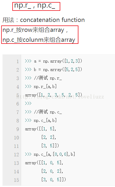
#预测
# np.c_  按照列来组合数组
Z = bdt.predict(np.c_[xx.ravel(),yy.ravel()])
#设置维度
Z = Z.reshape(xx.shape)

#画图
plot_coloes = "br"
class_names = "AB"

plt.figure(figsize=(10,5),facecolor="w")
#局部子图
plt.subplot(1,2,1)
plt.pcolormesh(xx,yy,Z,cmap=plt.cm.Paired)
for i,n,c in zip(range(2),class_names,plot_coloes):
    idx = np.where(y == i)
    plt.scatter(X[idx,0],X[idx,1],c=c,cmap=plt.cm.Paired,label=u"类别%s"%n)

plt.xlim(x_min,x_max)
plt.ylim(y_min,y_max)
plt.legend(loc="upper right")
plt.xlabel("x")
plt.ylabel("y")
plt.title(u"Adaboost分类结果,正确率为:%.2f%%"%(bdt.score(X,y)*100))
plt.savefig("Adaboost分类结果.png")

#获取决策函数的数值
twoclass_out = bdt.decision_function(X)
#获取范围
plot_range = (twoclass_out.min(),twoclass_out.max())
plt.subplot(1,2,2)
for i,n,c in zip(range(2),class_names,plot_coloes):
#直方图
    plt.hist(twoclass_out[y==i],bins=20,range=plot_range,
             facecolor=c,label=u"类别%s"%n,alpha=.5)
x1,x2,y1,y2 = plt.axis()
plt.axis((x1,x2,y1,y2*1.2))
plt.legend(loc="upper right")
plt.xlabel(u"决策函数值")
plt.ylabel(u"样本数")
plt.title(u"Adaboost的决策值")
plt.tight_layout()
plt.subplots_adjust(wspace=0.35)
plt.savefig("Adaboost的决策值.png")
plt.show()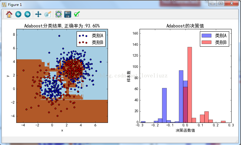

六、分类算法比较

#!/usr/bin/env python
# -*- coding:utf-8 -*-
# Author:ZhengzhengLiu

#分类算法比较

import numpy as np
import matplotlib as mpl
import matplotlib.pyplot as plt
from matplotlib.colors import ListedColormap

from sklearn.model_selection import train_test_split
from sklearn.preprocessing import StandardScaler
from sklearn.linear_model import LogisticRegressionCV
from sklearn.neighbors import KNeighborsClassifier
from sklearn.tree import DecisionTreeClassifier
from sklearn.ensemble import RandomForestClassifier,AdaBoostClassifier,GradientBoostingClassifier
from sklearn.datasets import make_moons,make_circles,make_classification    #生成月牙形、圆形和分类型的数据集

#解决中文显示问题
mpl.rcParams['font.sans-serif']=[u'simHei']
mpl.rcParams['axes.unicode_minus']=False

X,y = make_classification(n_features=2,n_redundant=0,n_informative=2,
                          random_state=1,n_clusters_per_class=1)
rng = np.random.RandomState(2)
X+=2*rng.uniform(size=X.shape)
linearly_separable = (X,y)

datasets = [make_moons(noise=0.3,random_state=0),
            make_circles(noise=0.2,factor=0.4,random_state=1),
            linearly_separable]

names = ["Nearest Neighbors", "Logistic","Decision Tree", "Random Forest", "AdaBoost", "GBDT"]
classifiers = [
    KNeighborsClassifier(3),
    LogisticRegressionCV(),
    DecisionTreeClassifier(max_depth=5),
    RandomForestClassifier(max_depth=5,n_estimators=10,max_features=1),
    AdaBoostClassifier(n_estimators=10,learning_rate=1.5),
    GradientBoostingClassifier(n_estimators=10,learning_rate=1.5)
]

#画图
figure = plt.figure(figsize=(27,9),facecolor="w")
i = 1
h = .02     #步长
for ds in datasets:
    X,y = ds
    X = StandardScaler().fit_transform(X)
    X_train,X_test,y_train,y_test = train_test_split(X,y,test_size=.4)

    x_min,x_max = X[:,0].min()-.5,X[:,0].max()+.5
    y_min,y_max = X[:,1].min()-.5,X[:,1].max()+.5

    xx,yy = np.meshgrid(np.arange(x_min,x_max,h),
                        np.arange(y_min,y_max,h))

    cm = plt.cm.RdBu
    cm_bright = ListedColormap(["r","b","y"])
    ax = plt.subplot(len(datasets),len(classifiers)+1,i)
    ax.scatter(X_train[:,0],X_train[:,1],c=y_train,cmap=cm_bright)
    ax.scatter(X_test[:,0],X_test[:,1],c=y_test,cmap=cm_bright,alpha=0.6)
    ax.set_xlim(xx.min(),xx.max())
    ax.set_ylim(yy.min(),yy.max())
    ax.set_xticks(())
    ax.set_yticks(())
    i+=1

    #画每个算法的图
    for name,clf in zip(names,classifiers):
        ax = plt.subplot(len(datasets),len(classifiers)+1,i)
        clf.fit(X_train,y_train)
        score = clf.score(X_test,y_test)
        if hasattr(clf,"decision_function"):
            Z = clf.decision_function(np.c_[xx.ravel(),yy.ravel()])
        else:
            Z = clf.predict_proba(np.c_[xx.ravel(),yy.ravel()])[:,1]
        Z = Z.reshape(xx.shape)
        ax.contourf(xx,yy,Z,cmap=cm,alpha=.8)
        ax.scatter(X_train[:,0],X_train[:,1],c=y_train,cmap=cm_bright)
        ax.scatter(X_test[:, 0], X_test[:, 1], c=y_test, cmap=cm_bright, alpha=0.6)
        ax.set_xlim(xx.min(), xx.max())
        ax.set_ylim(yy.min(), yy.max())
        ax.set_xticks(())
        ax.set_yticks(())
        ax.set_title(name)
        ax.text(xx.max()-.3,yy.min()+.3,("%.2f"%score).lstrip("0"),
                size=15,horizontalalignment="right")
        i+=1

#展示图
figure.subplots_adjust(left=.02,right=.98)
plt.savefig("分类算法比较.png")
plt.show()