吴恩达机器学习 EX3 作业 第二部分神经网络 前向传播 手写数字

2 神经网络前向传播

神经网络是一种很古老的算法，它最初产生的目的是制造能模拟大脑的机器。20世纪八九十年代比较火，后来支持向量机的兴起而逐渐衰落。21世纪第一个十年后期，由于计算机处理能力的显著提高，神经网络又火起来。
科学家希望模拟人的大脑，不同的接收器官(比如眼睛、鼻子、耳朵)接收信号，经过多个不同神经元处理，形成最终的信息

神经网络包含：一个输入层、一个输出层、多个隐藏层
如下图3层神经网络包含：一个输入层、一个隐藏层、一个输出层。前向传播过程见下图

2.1 作业介绍

在本练习的前一部分中，您实现了多类逻辑回归来识别手写数字。然而，逻辑回归只是一个线性分类器，不能形成更复杂的假设
在本部分练习中，您将使用与前面相同的训练集实现一个神经网络来识别手写数字。神经网络将能够表示形成非线性假设的复杂模型。这周，你们将使用我们已经训练过的神经网络的参数。您的目标是实现x前向传播算法来使用我们的权重进行预测。在下周的练习中，您将编写学习神经网络参数的反向传播算法。

2.2 导入模型和数据

导入模块

import matplotlib.pyplot as plt
import numpy as np
import scipy.io as scio

import displayData as dd # 绘制手写图形函数
import predict as pd # 预测函数

初始化数据

plt.ion()

# Setup the parameters you will use for this part of the exercise
input_layer_size = 400  # 20x20 input images of Digits
hidden_layer_size = 25  # 25 hidden layers
num_labels = 10         # 10 labels, from 0 to 9
                        # Note that we have mapped "0" to label 10

导入数据

data = scio.loadmat('ex3data1.mat')
X = data['X']
y = data['y'].flatten()
m = y.size

2.3 绘制数字图片函数(displayData.py)

import matplotlib.pyplot as plt
import numpy as np

def display_data(x):
    (m, n) = x.shape # 训练样本维度 (100, 400)
    # Set example_width automatically if not passed in
    example_width = np.round(np.sqrt(n)).astype(int) # 数字图片宽 20
    example_height = (n / example_width).astype(int) # 数字图片高 20
    # Compute the number of items to display
    display_rows = np.floor(np.sqrt(m)).astype(int) # 训练样本行数：10
    display_cols = np.ceil(m / display_rows).astype(int) # 训练样本列数：10 
    # Between images padding
    pad = 1 # 数字图片前后左右间隔为1px
    # Setup blank display 显示样例图片范围
    display_array = - np.ones((pad + display_rows * (example_height + pad),
                              pad + display_rows * (example_height + pad)))
    # Copy each example into a patch on the display array
    curr_ex = 0
    for j in range(display_rows):
        for i in range(display_cols):
            if curr_ex > m:
                break
            # Copy the patch
            # Get the max value of the patch
            max_val = np.max(np.abs(x[curr_ex]))#不明白为啥要除最大值，没看出差异
            # 开始一个个画出数字图
            display_array[pad + j * (example_height + pad) + np.arange(example_height),
                          pad + i * (example_width + pad) + np.arange(example_width)[:, np.newaxis]] = \
                          x[curr_ex].reshape((example_height, example_width)) / max_val
            curr_ex += 1

        if curr_ex > m:
            break

    # Display image
    plt.figure()
    plt.imshow(display_array, cmap='gray', extent=[-1, 1, -1, 1])
    plt.axis('off')

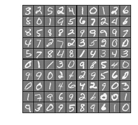
随机选择100数字图，并显示效果

# Randomly select 100 data points to display
rand_indices = np.random.permutation(range(m))
selected = X[rand_indices[0:100], :]

dd.display_data(selected)

2.4 加载提供已训练好参数的theta

data = scio.loadmat('ex3weights.mat')
theta1 = data['Theta1']
theta2 = data['Theta2']

显示theta

print('theta1.shape: ',theta1.shape, '\ntheta2.shape: ', theta2.shape)

theta1.shape:  (25, 401)
theta2.shape: (10, 26)

2.5 用神经网络训练的参数预测手写数字

sigmoid公式

sidmoid函数

def sigmoid(z):
    g = 1 / (1 + np.exp(-z))
    return g

预测函数predict.py

from sigmoid import *
def predict(theta1, theta2, x):
    # Useful values
    m = x.shape[0]
    num_labels = theta2.shape[0]

    # You need to return the following variable correctly
    p = np.zeros(m)

    a1 = np.c_[np.ones(m), x] 
    z2 = np.dot(a1, theta1.T)
    a2 = np.c_[np.ones(m),sigmoid(z2)]
    z3 = np.dot(a2, theta2.T)
    a3 = sigmoid(z3)
    p = np.argmax(a3, axis=1) + 1

    return p

调用预测函数预测并打印预测准确百分比，神经网络预测准确率97.52，较多分类逻辑回归要高好多

pred = predict(theta1, theta2, X)
print('Training set accuracy: {}'.format(np.mean(pred == y)*100))

Training set accuracy: 97.52

def getch():
    import termios
    import sys, tty

    def _getch():
        fd = sys.stdin.fileno()
        old_settings = termios.tcgetattr(fd)
        try:
            tty.setraw(fd)
            ch = sys.stdin.read(1)
        finally:
            termios.tcsetattr(fd, termios.TCSADRAIN, old_settings)
        return ch

    return _getch()

# Randomly permute examples
rp = np.random.permutation(range(m))
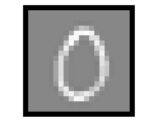
for i in range(m):
    print('Displaying Example image')
    example = X[rp[i]]
    example = example.reshape((1, example.size))
    dd.display_data(example)

    pred = pd.predict(theta1, theta2, example)
    print('Neural network prediction: {} (digit {})'.format(pred, np.mod(pred, 10)))

    s = input('Paused - press ENTER to continue, q + ENTER to exit: ')
    if s == 'q':
        break

Displaying Example image
Neural network prediction: [0.] (digit [0.])
Paused - press ENTER to continue, q + ENTER to exit: 
Displaying Example image
Neural network prediction: [0.] (digit [0.])
Paused - press ENTER to continue, q + ENTER to exit: 
Displaying Example image
Neural network prediction: [0.] (digit [0.])
Paused - press ENTER to continue, q + ENTER to exit: 
Displaying Example image
Neural network prediction: [0.] (digit [0.])
Paused - press ENTER to continue, q + ENTER to exit: 
Displaying Example image
Neural network prediction: [0.] (digit [0.])
Paused - press ENTER to continue, q + ENTER to exit: 
Displaying Example image
Neural network prediction: [0.] (digit [0.])
Paused - press ENTER to continue, q + ENTER to exit: 
Displaying Example image
Neural network prediction: [0.] (digit [0.])
Paused - press ENTER to continue, q + ENTER to exit: 
Displaying Example image
Neural network prediction: [0.] (digit [0.])
Paused - press ENTER to continue, q + ENTER to exit: q

前一篇 吴恩达机器学习 EX3 作业 第一部分多分类逻辑回归 手写数字
后一篇 吴恩达机器学习 EX4 作业 神经网络反向传播 手写数字