LeNet5—论文及源码阅读

LeNet5实现图像分类

🐬 目录:

• 一、概论
• 二、论文选读
• 三、源码精读
  1. 所用数据集介绍
  2. LeNet5模型网络构建
  3. LeNet5模型训练
  4. 测试代码
• 四、参考资料

---

一、概论

LeNet-5是一种经典的卷积神经网络结构，于1998年投入实际使用中。该网络最早应用于手写体字符识别应用中。普遍认为，卷积神经网络的出现开始于LeCun等提出的LeNet网络，可以说LeCun等是CNN的缔造者，而LeNet则是LeCun等创造的CNN经典之作。

二、论文选读

论文： 《Gradient-Based Learning Applied to Document Recognition》

---

LeNet-5 comprises seven layers, not counting the input, all of which contain trainable parameters (weights). The input is a 32×32 pixel image.

理解： LeNet5共包含7层，输入为32×32像素的图片，如下图所示：

---

---

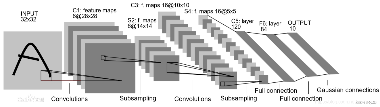
Layer C1 is a convolutional layer with six feature maps.Each unit in each feature map is connected to a 5✖5 neigh-borhood in the input.

理解： C1 层是卷积层，使用 6 个 5×5 大小的卷积核，padding=0，stride=1进行卷积，得到 6 个 28×28 大小的特征图：32-5+1=28

---

---

Layer S2 is a subsampling layer with six feature maps of size 14×14. Each unit in each feature map is connected to a 2×2 neighborhood in the corresponding feature map in C1.The four inputs to a unit in S2 are added, then multiplied by a trainable coefficient, and then added to a trainable bias.The result is passed through a sigmoidal function.

理解： S2 层是降采样层，使用 6 个 2×2 大小的卷积核进行池化，padding=0，stride=2，得到 6 个 14×14 大小的特征图：28/2=14。S2 层其实相当于降采样层+激活层。先是降采样，然后激活函数 sigmoid 非线性输出。先对 C1 层 2x2 的视野求和，然后进入激活函数。

---

---

Layer C3 is a convolutional layer with 16 feature maps.Each unit in each feature map is connected to several 5×5 neighborhoods at identical locations in a subset of S2’s feature maps.
The first six C3 feature maps take inputs from every contiguous subsets of three feature maps in S2. The next six take input from every contiguous subset of four. The next three take input from some discontinuous subsets of four. Finally, the last one takes input from all S2 feature maps.

理解： C3 层是卷积层，使用 16 个 5×5xn 大小的卷积核，padding=0，stride=1 进行卷积，得到 16 个 10×10 大小的特征图：14-5+1=10。
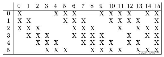
16 个卷积核并不是都与 S2 的 6 个通道层进行卷积操作，如下图所示，C3 的前六个特征图（0,1,2,3,4,5）由 S2 的相邻三个特征图作为输入，对应的卷积核尺寸为：5x5x3；接下来的 6 个特征图（6,7,8,9,10,11）由 S2 的相邻四个特征图作为输入对应的卷积核尺寸为：5x5x4；接下来的 3 个特征图（12,13,14）号特征图由 S2 间断的四个特征图作为输入对应的卷积核尺寸为：5x5x4；最后的 15 号特征图由 S2 全部(6 个)特征图作为输入，对应的卷积核尺寸为：5x5x6。

---

---

Layer S4 is a subsampling layer with 16 feature maps of size 5×5. Each unit in each feature map is connected to a 2×2 neighborhood in the corresponding feature map in C3.

理解： S4 层与 S2 一样也是降采样层，使用 16 个 2×2 大小的卷积核进行池化，padding=0，stride=2，得到 16 个 5×5 大小的特征图：10/2=5。

---

---

Layer C5 is a convolutional layer with 120 feature maps.Each unit is connected to a 5×5 neighborhood on all 16 of S4’s feature maps.

理解： C5 层是卷积层，使用 120 个 5×5x16 大小的卷积核，padding=0，stride=1进行卷积，得到 120 个 1×1 大小的特征图：5-5+1=1。即相当于 120 个神经元的全连接层。
值得注意的是，与C3层不同，这里120个卷积核都与S4的16个通道层进行卷积操作。

---

---

Layer F6 contains 84 units (the reason for this number comes from the design of the output layer, explained below) and is fully connected to C5.
units in layers up to F6 compute adot product between their input vector and their weigh tvector, to which a bias is added.
then passed through a sigmoid squashing function

理解： F6 是全连接层，共有 84 个神经元，与 C5 层进行全连接，即每个神经元都与 C5 层的 120 个特征图相连。计算输入向量和权重向量之间的点积，再加上一个偏置，结果通过 sigmoid 函数输出。

---

---

the output layer is composed of Euclidean RBFunits, one for each class, with 84 inputs each.

理解 :最后的 Output 层也是全连接层，是 Gaussian Connections，采用了 RBF 函数（即径向欧式距离函数），计算输入向量和参数向量之间的欧式距离（目前已经被Softmax 取代）。

三、源码精读

📡 实现效果

3.1 所用数据集介绍

CIFAR-10 是由 Hinton 的学生 Alex Krizhevsky 和 Ilya Sutskever 整理的一个用于识别普适物体的小型数据集。一共包含 10 个类别的 RGB 彩色图 片：飞机（ airplane ）、汽车（ automobile ）、鸟类（ bird ）、猫（ cat ）、鹿（ deer ）、狗（ dog ）、蛙类（ frog ）、马（ horse ）、船（ ship ）和卡车（ truck ）。图片的尺寸为 32×32 ，数据集中一共有 50000 张训练圄片和 10000 张测试图片。

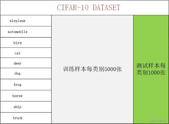
数据集分为五个训练batches和一个测试batch，每个batch有10000张图像。测试batch包含从每个类中随机选择的1000个图像。训练batches以随机顺序包含剩余的图像，但有些训练batches可能包含一个类的图像多于另一个类的图像。在它们之间，训练batches包含来自每个类的5000张图像

3.2 LeNet5模型网络构建

class LeNet(nn.Module):
    def __init__(self):
        super(LeNet, self).__init__()	#调用父类nn.Module中的init方法对属性进行初始化
        self.conv1 = nn.Conv2d(3, 16, 5)	 
        self.pool1 = nn.MaxPool2d(2, 2)
        self.conv2 = nn.Conv2d(16, 32, 5)
        self.pool2 = nn.MaxPool2d(2, 2)
        self.fc1 = nn.Linear(32*5*5, 120)
        self.fc2 = nn.Linear(120, 84)
        self.fc3 = nn.Linear(84, 10)

根据论文描述，LeNet5共包含7层。上述代码作用为初始化属性，为后续forward函数的调用做准备，上述代码中所用基本函数定义，查阅pytorch官方文档如下表所示：

函数	介绍
nn.Conv2d(3,16,5)	torch.nn.Conv2d(in_channels = 3, out_channels = 16, kernel_size = 5 * 5, stride=1, padding=0, dilation=1, groups=1, bias=True, padding_mode=‘zeros’, device=None, dtype=None)
nn.MaxPool2d(2, 2)	torch.nn.MaxPool2d(kernel_size = 2 * 2, stride=None, padding=0, dilation=1, return_indices=False, ceil_mode=False
nn.Linear(32 * 5 * 5, 120)	torch.nn.Linear(in_features = 32 * 5 * 120, out_features = 120, bias=True, device=None, dtype=None)

3.3 LeNet5模型训练

🐢 3.3.1 下载数据集

    #逐channel的对图像均值/方差进行标准化。可以加快模型的收敛
    transform = transforms.Compose(
        [transforms.ToTensor(),
         transforms.Normalize((0.5, 0.5, 0.5), (0.5, 0.5, 0.5))])
  
    # 50000张训练图片
    # 第一次使用时要将download设置为True才会自动去下载数据集
    train_set = torchvision.datasets.CIFAR10(root='./data', train=True,
                                             download=True, transform=transform)
    train_loader = torch.utils.data.DataLoader(train_set, batch_size=36,
                                               shuffle=True, num_workers=0)
                                               
    # 10000张验证图片
    # 第一次使用时要将download设置为True才会自动去下载数据集
    val_set = torchvision.datasets.CIFAR10(root='./data', train=False,
                                           download=False, transform=transform)

🐢 3.3.2 加载数据集

Data loader. Combines a dataset and a sampler, and provides an iterable over the given dataset.

train_loader = torch.utils.data.DataLoader(train_set, batch_size=36,
                                               shuffle=True, num_workers=0)
val_loader = torch.utils.data.DataLoader(val_set, batch_size=5000,
                                             shuffle=False, num_workers=0)

🐢 3.3.3 训练LeNet5网络，学习参数

    for epoch in range(5):  # loop over the dataset multiple times

        running_loss = 0.0
        for step, data in enumerate(train_loader, start=0):
            # get the inputs; data is a list of [inputs, labels]
            inputs, labels = data

            # zero the parameter gradients
            optimizer.zero_grad()
            # forward + backward + optimize
            outputs = net(inputs)
            loss = loss_function(outputs, labels)
            loss.backward()
            optimizer.step()

            # print statistics
            running_loss += loss.item()	#tensor to Int
            if step % 500 == 499:    # print every 500 mini-batches
                with torch.no_grad():
                    outputs = net(val_image)
                    predict_y = torch.max(outputs, dim=1)[1]
                    accuracy = torch.eq(predict_y, val_label).sum().item() / val_label.size(0)

                    print('[%d, %5d] train_loss: %.3f  test_accuracy: %.3f' %
                          (epoch + 1, step + 1, running_loss / 500, accuracy))
                    running_loss = 0.0

    print('Finished Training')

🐢 3.3.4 保存模型权重

    save_path = './Lenet.pth'
    torch.save(net.state_dict(), save_path)     #获取模型的参数，而不保存结构

3.4 测试代码

import torch
import torchvision.transforms as transforms
from PIL import Image

from model import LeNet


def main():
    transform = transforms.Compose(
        [transforms.Resize((32, 32)),
         transforms.ToTensor(),
         transforms.Normalize((0.5, 0.5, 0.5), (0.5, 0.5, 0.5))])

    classes = ('plane', 'car', 'bird', 'cat',
               'deer', 'dog', 'frog', 'horse', 'ship', 'truck')

    net = LeNet()
    net.load_state_dict(torch.load('Lenet.pth'))

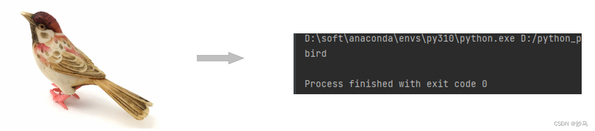
    im = Image.open('img.png')
    im = transform(im)  # [C, H, W]
    im = torch.unsqueeze(im, dim=0)  # [N, C, H, W]

    with torch.no_grad():
        outputs = net(im)
        predict = torch.max(outputs, dim=1)[1].numpy()
    print(classes[int(predict)])


if __name__ == '__main__':
    main()

四、参考资料

这可能是神经网络 LeNet-5 最详细的解释了！